Screened Waves

a jigsaw puzzle-like basis set for 1-particle wavefunctions

Dimitar Pashov, KCL

IIIDQS, 16 May 2019, STFC Daresbury

Idea

Construct a set of functions which almost solve the 1-particle Schrödinger/Dirac equation for real potentials
without spending effort equivalent to or grater than actually solving it.

Without global matrix operations: multiplication, inversion, diagonalisation, decompositions, etc...
Without global energy scan and functions reconstructions

The function set shall

preserve the rigour and accuracy of augmented methods
be mimimal, reasonably complete and not overcomplete
be reasonably short ranged (system dependent), allowing scalable integration
take advantage of low expansion cutoffs of the PAW scheme (described in Mark's intro to LMTO talk).

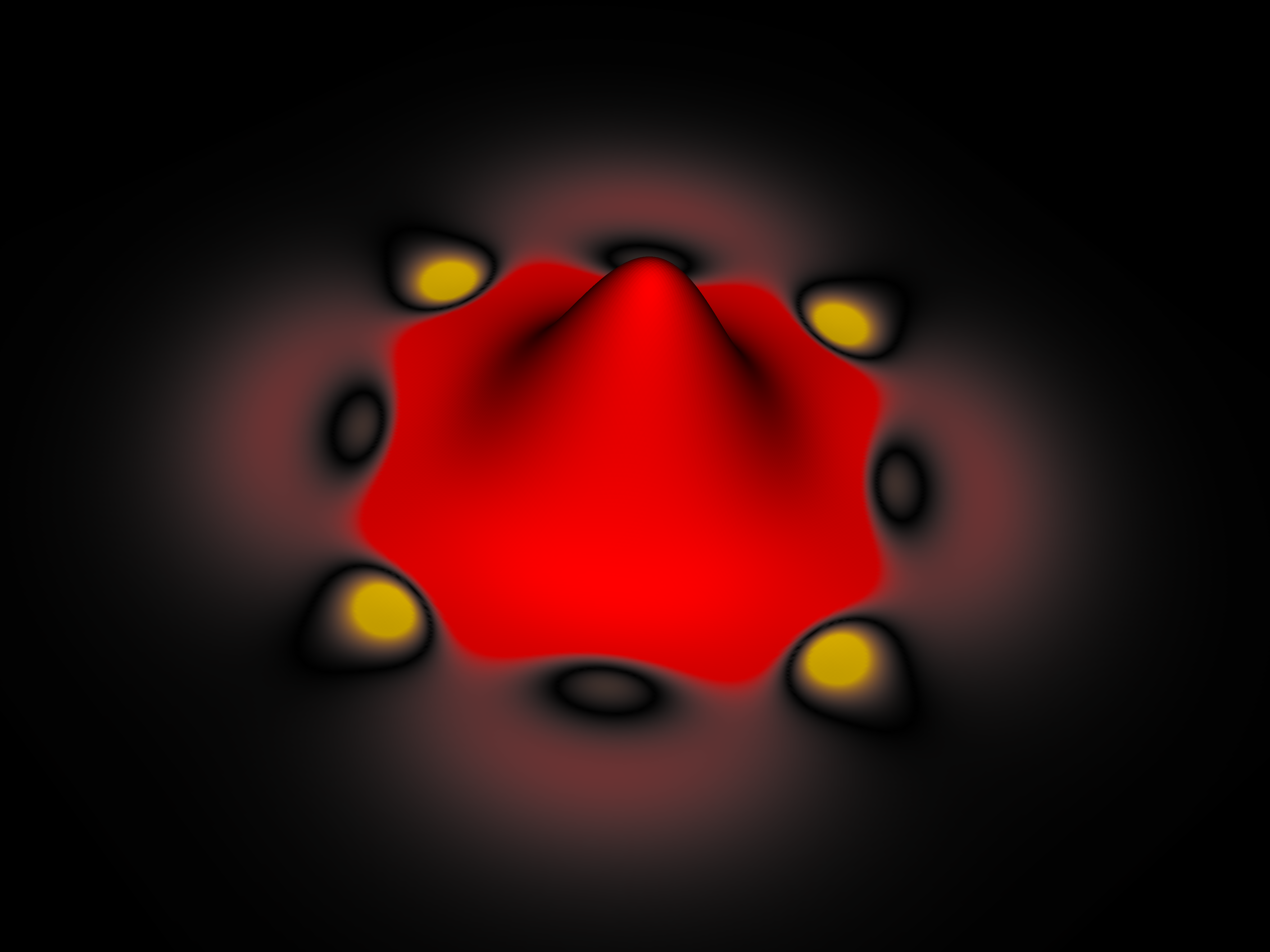
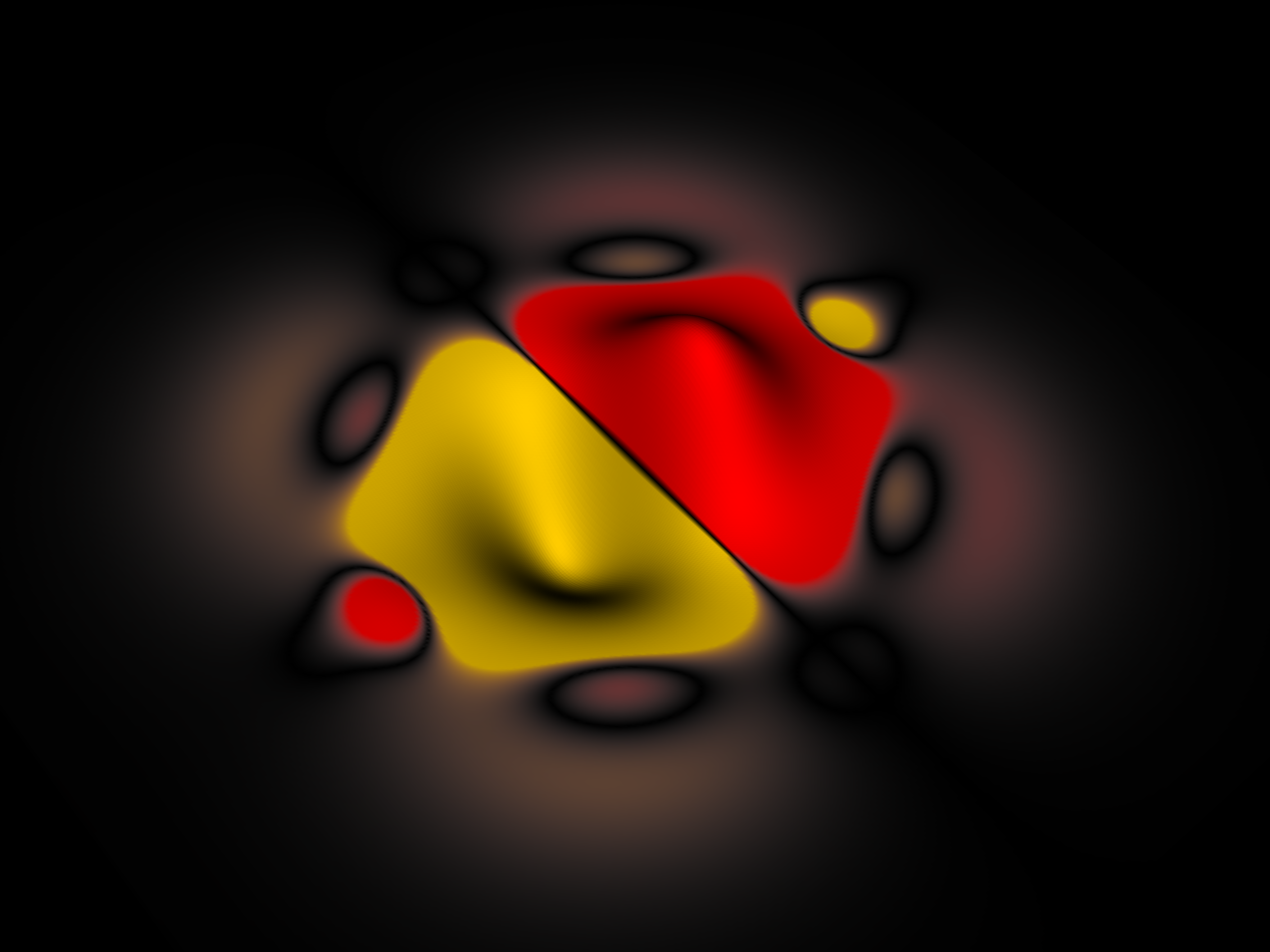
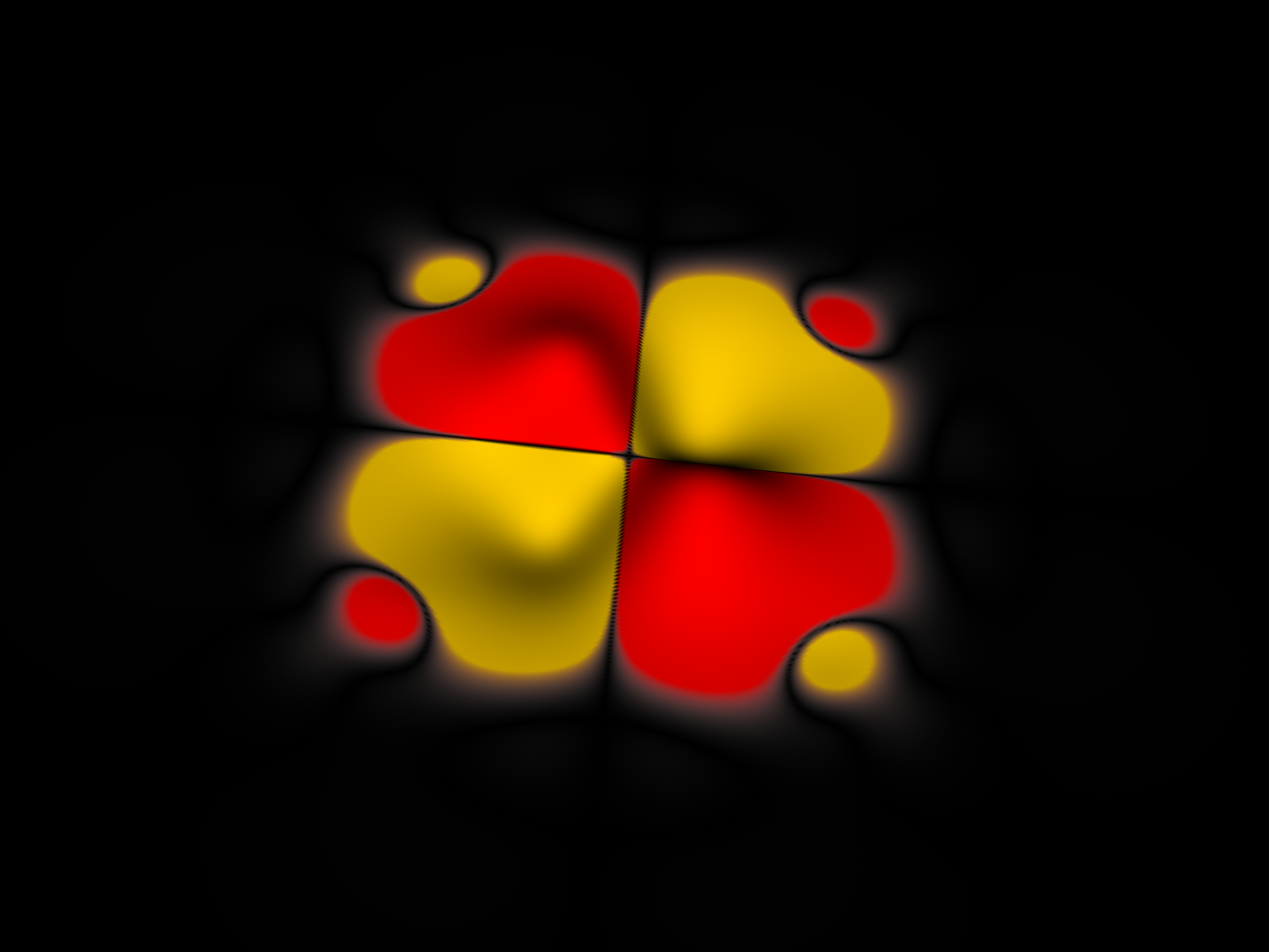
s-type function (interactve isosurface model)

QSGW Si bandstructure

Short deviation to explain yesterday's unfortunate confusion on the LiF example

blm --gw --nkgw=5 --nk=8 --nit=20 --gmax=9.8 --ctrl=ctrl init.lif

interpolating 8×8×8 mesh from 5×5×5 sigma file on a tiny system, potentially dangerous (as we saw yesterday with Brian), terribly false gap of 2.44 eV, parallels with 2×2×2 Si bands picture (unscreened case):

vs

blm --gw --nkgw=5 --nk=5 --nit=20 --gmax=9.8 --ctrl=ctrl init.lif

interpolating 5×5×5 mesh from 5×5×5 sigma more reliable because points match (bar the Γ point, which always gets a special treatment): bandgap: 16.65 eV

Truncated QSGW NiO band gap

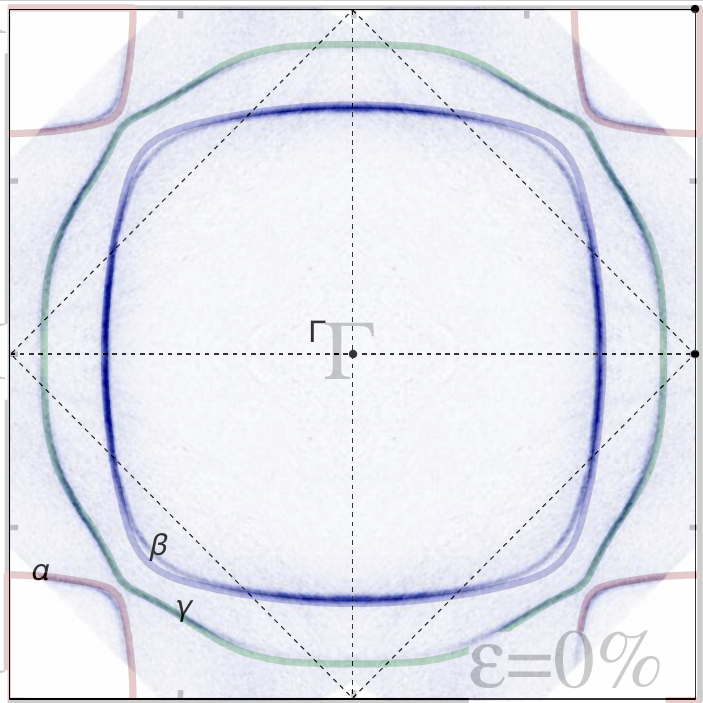
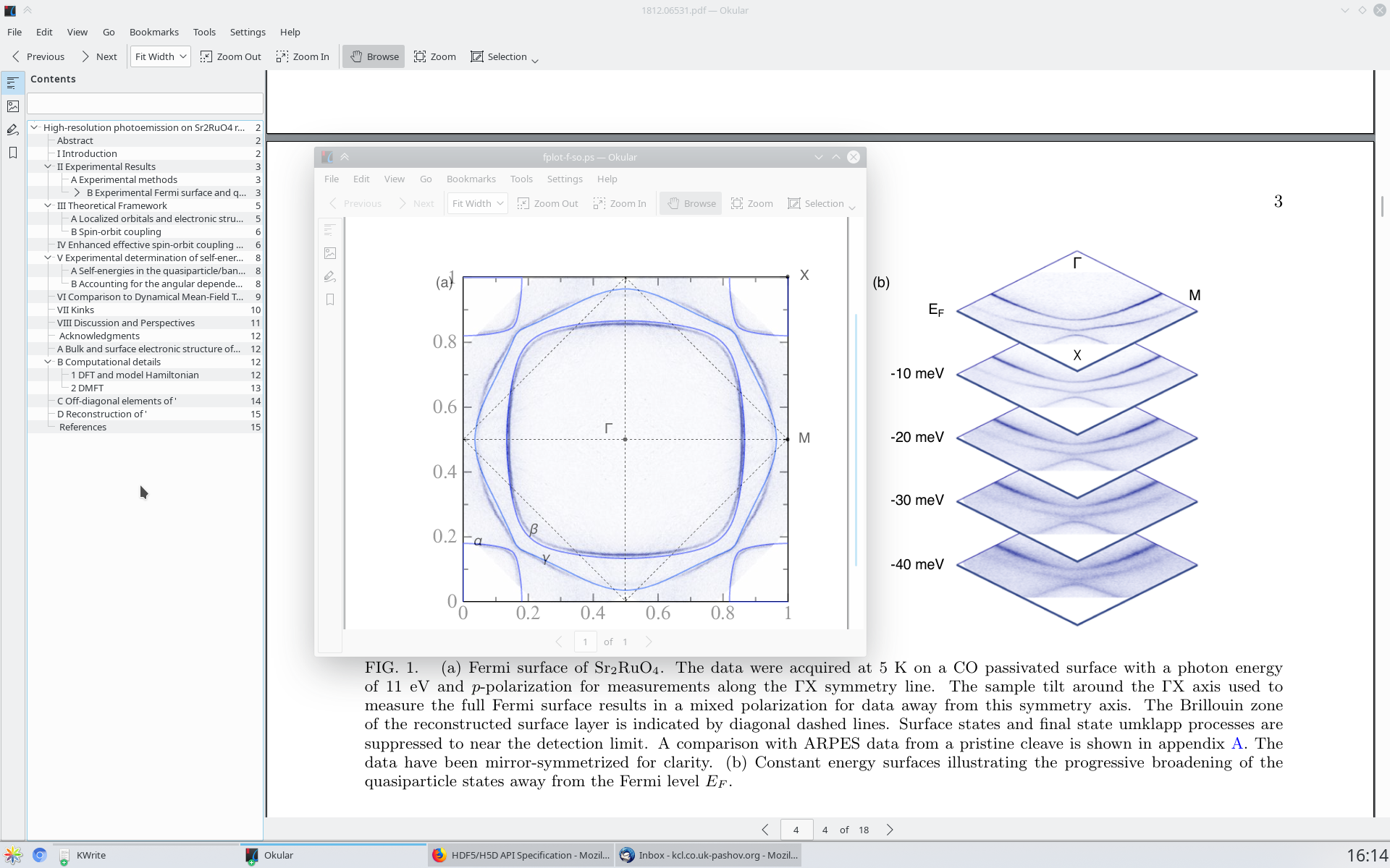
Strontium Ruthenate Fermi surface (8×8×8 mesh)

experiment, screened (overlay) and unscreened basis

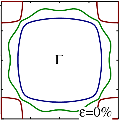
Strontium Ruthenate 6×6×6 screened basis

Screened LMTO in a coconutshell

$H$: $h.Y$; $J$: $j.Y$; $Y$: spherical harmonics; $I$: identity (sometimes product of Kronecker deltas)

$H_{RLR'L'}$ : The $L'$ component of a function $H_L$ centered on site $R$ evaluated at site $R'$.

\[ H_{RLR'L'} = H_{L} I_{RLR'L'} + S_{RLR'L'} J_{L'} . (1-I_{RR'}) \] (in smooth H case there is additional short ranged $P_{kL}$ expansion of $H^{sm}-H$ which is ignored here for clarity) Here $S_{RLR'L'}$ is an expansion coefficient such that $H_{RL(r)} = \sum_{L'} S_{RLR'L'} J_{L'R}$ Let's concretise for sphere surfaces only and rescale by $1/H_{L'}$ rather than $1/H_{L}$ to preserve the original symmetry of $J$ $\left(\right.$now $\left. J/H\right)$, $H_{L} I_{RLR'L'} / H_{L'} == H_{L} I_{RLR'L'} / H_{L} == I_{RLR'L'}$ for spheres of the same size anyway. \[ H_{RLR'L'}/H_{L'} = I_{RLR'L'} + S_{RLR'L'} J_{L'}/H_{L'} . (1-I_{RR'}) \]

Let's shorten $J_{L}/H_{L}$ to just $\alpha_{L}$, it is a diagonal in matrix form. With $\mathrm{H} \equiv H_{RLR'L'}/H_{L'}$ and other appropriate aliasing: \[ \mathrm{H} = \mathrm{I} + \mathrm{S} \alpha \] Now request functions $E_{RL}$ made of combinations of H functions such that they evaluate to unit on their own $R$ centered spheres but vanish at all other spheres (i.e. I_{RLR'L'}). The combination coefficients $B$ are to be found. \[ E_{RLR'L'} = H_{L} δ_{RR'} δ_{LL'} = \sum_{R''L''} B_{RLR''L''} H_{R''L''R'L'} \] to avoid messy indices let's alias $\mathrm{E} \equiv E_{RLR'L'}/H_{L'} \equiv \mathrm{I}$, then: \[ \mathrm{E} = \mathrm{B} \mathrm{H}; \quad \mathrm{B} = \mathrm{E} \mathrm{H^{-1}} = (\mathrm{I} + \mathrm{S} \alpha)^{-1} = a^{-1} (a^{-1} + \mathrm{S})^{-1} \]

We do have kinks on the sphere boundaries due to the augmentation functions mathing the value (and curvature) only. \begin{align} & K_{1,RLR'L'} = & dE_{1,RLR'L'} - & d\phi_{1,RLR'L'} \\ & K_{2,RLR'L'} = & dE_{2,RLR'L'} - & d\phi_{2,RLR'L'} \\ & : : & & : \\ & K_{n,RLR'L'} = & dE_{n,RLR'L'} - & d\phi_{n,RLR'L'} \end{align} these can be straightened out by interpolating to 0 kink matrix using functions at 2 or more energies. Example with Lagrange weights: \[ F = \sum_{e=1}^n \left( \prod_{k=1;k/=e}^n K_k . (K_k - K_e)^{-1} \right) E_e \]

The same can also be derived (with more difficulty) from the Vandermonde matrix: \begin{align} F = (I\, 0\, 0) & (K_1^0 K_1^1 ... K_1^n)^{-1} & E_1 \\ & (K_2^0 K_2^1 ... K_2^n) & E_2 \\ & : : ::: : & : \\ & (K_n^0 K_n^1 ... K_n^n) & E_n \\ \end{align} For the simple case of 2 energies: \[ F = K_2 (K_2 - K_1)^{-1} E_1 - K_1 (K_2 - K_1)^{-1} E_2 \] adding more linearisation energies sharpens the window of accuracy, (improves significntly between the energies and worsens as much outside of it).