Implementation of the GW Approximation
Table of Contents
- Introduction
- How the 1-particle and many-particle codes synchronise
- Analysis of many-body spectral functions
- Other Resources
Introduction
Questaal’s has two forms of GW implemented: a classic implementation (master branch) and a modern one (gw-speedup branch). The modern form is far more efficient than the classic one, and it also has multiple levels of parallelization while the classic code has OMP parallelization only. Both classic and modern forms consist of a heterogeneous set of executables which are run by shell scripts. In the modern code, the script is called lmgw.sh. There is a user guide for it, as well as a tutorial that offers some detail how to run lmgwsh on high performance architectures. See the basic tutorial demonstrating its use in Si, and another tutorial for elemental iron, and also this tutorial for calculating the dielectric function.
The shell script for the classic code is called lmgwsc. Both the classic and modern versions have an implementation of the Qusiparticle Self-Consistent GW approximation (QSGW). In contrast to the usual implementation of GW the full self-energy matrix Σ is calculated and “quasiparticlized:” coupling one-electron states i and j, is evaluated at the one-particle energies and , and the average value is taken. This results in a static but orbital-dependent potential, a “quasiparticlized” derived from , and defines a one-particle hamiltonian which is the analog of the LDA or Hartree-Fock one-particle hamiltonian with substituting for .
The new is used to mke a new , and the process is iterated until stops changing. This is quasiparticle self-consistency.
QSGW theory is an elegant way to find the optimum noninteracting hamiltonian for GW calculations. It is vastly better than basing on the LDA, as is customary, albeit at some computational cost. A particularly valuable property of this optimum starting point is that the peaks of the interacting Green’s function G coincide with the poles of . The eigenfunctions of are as close as possible to those of G, by construction. What are true poles in get broadened by the interactions, so quasiparticles lose weight. Thus the density-of-states, or spectral function, is composed of a superposition of δ-functions for , but are broadened for G. Also the eigenvalues acquire an imaginary part, making the QP lifetime finite.
In QSGW theory and G are closely linked. Associated with the two kinds of G are two kinds of density-of-states (DOS). There is “noninteracting” or “coherent” DOS, namely the spectral function of which is associated with DOS in one-particle description, and is what is typically calculated by a band program such as lmf. There is also the true DOS (spectral function of G) which is approximately what is approximately measured by e.g. a photoemission experiment. The GW package has a facility to generate both kinds of DOS through the normal lmf process for the noninteracting DOS or by analyzing the spectral functions for the interacting case.
A detailed description of QSGW theory and the way in which Questaal implements it can be found in the references in “Other Resources” below.
In the classic code (and as of this writing the classic code only), the GW approximation is implemented in the traditional form: as a 1-shot perturbation to the LDA and as quasiparticle self-consistent GW (QSGW). In 1-shot mode, the diagonal part of Σ is evaluated at the one-particle (usually LDA) energies, yielding a correction to the LDA levels in 1st order perturbation theory. You can find a tutorial on this page. At present, the modern code does not have a one-shot version of GW.
How the 1-particle and many-particle codes synchronise
The GW package comprise a separate set of codes from the density-functional code, lmf. It uses the single-particle basis set of lmf to calculate the screened coulomb interaction W and the self-energy, Σ=iGW.
Thus, the GW package handles the many-body part, lmf the 1-body part. The two connect through special purpose interfaces: lmfgwd sets up the inputs needed by GW, supplying information about the wave functions in the augmentation spheres and in the interstitial. The GW part estimates shifts in QP levels and makes the quasiparticlized . Apart from these linkages, the GW package is completely separate from lmf. The GW package has a separate input file, GWinput and does not depend on the ctrl file lmf and lmfgwd use; only on the eigenfunctions they generate.
In reality the GW package makes . lmf can read this potential and add it to the LDA hamiltonian. This construction enables lmf to do the same kinds of calculations it performs with the LDA potential.
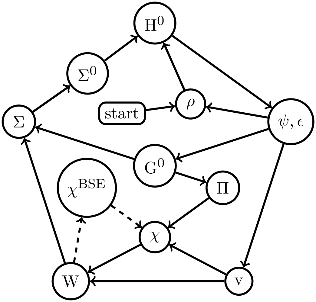
The QSGW flowchart is shown in the Figure. Initially lmf reads a trial charge density ρ (start) and makes a self-consistent ρ, which in DFT is sufficient to make a one-body H0. This is sufficient to start the QSGW cycle.
Both the classic and modern implementations perform the following steps
- lmfgwd constructs this H0 (initially H0=HDFT) to make eigenfunctions and eigenvalues (ψ, ε), which is sufficient to make G0 (in practice G0 is never calculated).
- Matrix elements of the Hartree potential are made (V).
- The bare polarizability (Π) is made.
- Π is combined with V to make the susceptibility χ and the RPA screened coulomb interaction (W).
- At this stage there is an option to improve on W by adding a vertex (χBSE).
- W is (formally) convolved with G0 to make the self-energy Σ(ω).
- Σ(ω) is quasiparticlized to make a static, but spatially nonlocal self-energy Σ0.
- lmf can be run again, now with a potential added to . lmf can iterate until the density is self-consistent (an inner self-consistent loop) and the entire cycle repeated until stops changing (outer loop).
In the classic code these steps are managed by script lmgw; lmgwsc is a higher level script that calls lmgw and cycles through outer loops until self-consistency is reached.
Note that when making the density self-consistent, in is kept frozen, while is updated. So there is an inexact cancellation of these two terms until self-consistency in is reached.
In the modern implementation, the same steps are taken, through script lmgw.sh. It differs from lmgw in that the calculation of W and Σ are performed in one large loop, to avoid writing large W files to disk.
Operation of lmfgwd
lmfgwd generates the same H0 as lmf, but its purpose is to create files needed for the GW cycle. After setting up the potential it prompts for a job, which tells lmfgwd what to do.
- Job −1 generates a GWinput and exits. The structure of this file is documented on this page. lmfgwd will make a reasonable GWinput, but it should be kept in mind that this file is only a template and it should be checked. Many of tags written to GWinput can be read from tags in the GW category of the ctrl file. (While tags in GWinput and the ctrl files are kept separate, this switch generates a GWinput that synchronises with the ctrl file.) Particularly important are QpGcut_cou and the k mesh (n1n2n3). Execution time is sensitive to both, so they are not given conservative values.
- Job 0 is an ‘initializer’ mode. It creates several input files the GW package requires: SYMOPS, LATTC, CLASS, NLAindx, ldima
- Job 1 generates files required by the GW package (e.g. eigenfunctions, eigenvalues, and wave function information)
- Job −2 performs sanity checks on GWinput
Even while the GW package is independent of lmf, the GWinput file is complicated and in practice almost always autogenerated by lmfgwd. What lmfgwd writes to GWinput is modified by contents in the ctrl file. lmfgwd reads a special GW category from the ctrl file; through tags in this category you can set some of the parameters it writes into GWinput .
Analysis of many-body spectral functions
A pair of executables spectral and lmfgws are included in the Questaal suite. They are postprocessing tools used to analyze spectral functions made by the GW package, derived by either individual QP levels or integrated over the Brillouin zone to make the interacting density-of-states. See this page for a tutorial on spectral functions.
Other Resources
See this tutorial for a basic introduction to doing a QSGW calculation.
This is Questaal’s main methods paper, which includes a detailed discussion of GW and QSGW:
Dimitar Pashov, Swagata Acharya, Walter R. L. Lambrecht, Jerome Jackson, Kirill D. Belashchenko, Athanasios Chantis, Francois Jamet, Mark van Schilfgaarde, Questaal: a package of electronic structure methods based on the linear muffin-tin orbital technique, Comp. Phys. Comm. 249, 107065 (2020).
This paper presents the first description of an all-electron GW implementation in a mixed basis set:
T. Kotani and M. van Schilfgaarde, All-electron GW approximation with the mixed basis expansion based on the full-potential LMTO method, Sol. State Comm. 121, 461 (2002).
These papers established the framework for QuasiParticle Self-Consistent GW theory:
Sergey V. Faleev, Mark van Schilfgaarde, Takao Kotani, All-electron self-consistent GW approximation: Application to Si, MnO, and NiO, Phys. Rev. Lett. 93, 126406 (2004);
M. van Schilfgaarde, Takao Kotani, S. V. Faleev, Quasiparticle self-consistent GW theory, Phys. Rev. Lett. 96, 226402 (2006)
Questaal’s GW implementation is based on this paper:
Takao Kotani, M. van Schilfgaarde, S. V. Faleev, Quasiparticle self-consistent GW method: a basis for the independent-particle approximation, Phys. Rev. B76, 165106 (2007)
This paper shows all-electron results from LDA-based GW, and its limitations:
M. van Schilfgaarde, Takao Kotani, S. V. Faleev, Adequacy of Approximations in GW Theory, Phys. Rev. B74, 245125 (2006)