Zeeman Field Tutorial
Hazard: this page has not been carefully worked out, especially the description of the Stoner parameter may not be accurate.
You can add to the crystal potential an external magnetic field inside each augementation sphere, in the ASA program lm and full-potential program lmf. Use token BFIELD to tell lm or lmf that a field is to be read. The calculation must be spin polarized, e.g. the ctrl file should contain:
HAM    NSPIN=2 BFIELD=2
...
BFIELD=1 allows the field to point in any direction; BFIELD=2 restricts the field to the z axis. The former case generates a noncollinear hamiltonian; the latter is spin diagonal. (The hamiltonian may also be noncollinear for another reason, e.g. spin-orbit coupling is turned on.) Note: lmf does not as yet generate noncollinear output densities. Self-consistent calculations with noncollinear B fields are not possible; also the total energy is not trustworthy if B is not along the z axis.
By selecting BFIELD nonzero, you are telling lm or lmf that a (site-dependent) Zeeman field is to be added. Besides adding the tag HAM_BFIELD to the ctrl file you must create a file bfield.ext. It is a simple ASCII file described here bfield.ext contains the size of the magnetic field, one line for each site, three numbers x,y,z for components of B. (The file must always contain three components Bx. By Bz even if BFIELD=2.) If this file is omitted, the program will run but no field will be added.
The GdN test case (part of the test suite) is an instructive example. In the top-level directory, run this test:
fp/test/test.fp gdn
This test combines the LDA+U hamiltonian with spin-orbit coupling. Bands are calculated for that case; then a magnetic field of 0.25 eV=0.037/2 Ry is added to the Gd site and the bands are recalculated. GdN has two atoms and file bfield.gdn reads:
0 0 .037/2
0 0 0
The test below generates files bnds.bfield.gdn and bnds.nobfield.gdn. To analyze the bands you need to use a graphics package. If you have the fplot package installed, you can draw the picture shown below comparing the two cases, by invoking the following commands after running the test:
echo -8,8,5,10 | plbnds -fplot -ef=0 -scl=13.6 -lbl=L,G,X,W,G -dat=blue bnds.nobfield.gdn
echo -8,8,5,10 | plbnds -fplot -ef=0 -scl=13.6 -lbl=L,G,X,W,G -dat=dat  bnds.bfield.gdn
mv plot.plbnds plot.plbnds~
echo "% char0 colr=3,bold=4,clip=1,col=1,.2,.3" >>plot.plbnds
echo "% char0 colb=2,bold=2,clip=1,col=.2,.3,1" >>plot.plbnds
awk '{if ($1 == "-colsy") {sub("-qr","-lt {colr} -qr");print;sub("dat","blue");sub("colr","colb");print} else {print}}' plot.plbnds~ >>plot.plbnds
fplot -disp -f plot.plbnds
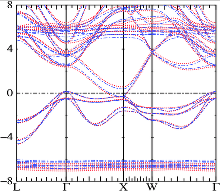
In the figure, blue bands are LDA+U results. Because spin-orbit coupling is included both minority and majority spin bands appear. You can see majority Gd f states near -6.5 eV, and minority f states near +5.5 eV. Gd d states are spin-split by the exchange-correlation field originating from spin splitting of the Gd f states; majority and minority d states are found near 2.5 eV and 3.5 eV, respectively, at the Γ point.
Red bands use the same potential as the LDA+U case, except that a Bz field of magnitude 0.5 eV was added to the Gd site. Bz causes the the following shifts:
- The majority f shifts down by ~0.22 eV, and the minority f states shift up by ~0.27 eV. States that are purely atomic like and are little affected by the kinetic energy will be shifted by the Zeeman field, ±B/2. This is the case for Gd f orbitals.
- The majority d states at Γ shift down by ~0.16 eV; the minority d states shift up by ~0.20 eV.
- The As p states, in the (-4,0) eV range, are only slightly shifted.
Longitudinal susceptibility
The magnetic susceptibility is the system’s magnetic response to an external magnetic field:
or
δM itself can be obtained from a derivative of the total energy:
Thus
and
In linear response theory, can be written as a sum of a noninteracting part and an interacting part
The kernel is often associated with the “Stoner parameter.” It is typically about 1 eV in 3d transition metals. The noninteracting part is connected with the induced magnetization of the noninteracting system, i.e.
where is the magnetization induced by without taking into account the internal potential shifts that cause. In the density-functional context, can be obtained from an initially self-consistent potential , which is generated in the absence of an external field. is then the change in for the potential . In practice this is obtained by evaluating the change in from the change in output density of a 1-shot calculation with potential .
You can use lmf to apply a field and calculate E_LDA and δ_M as a function of B. By comparing self-consistent and 1-shot calculations you can in principle also obtain I. The example below does this in an approximate way for Fe, using input file fp/test/ctrl.felz. Note: a proper calculation of I would require a supercell large enough that the interactions between external B-fields would be sufficiently small. (I is a local function of r in density functional theory; thus I is a site-diagonal matrix.) Here we only consider a single atom cell. The interactions are not small, and I is underestimated. The results below were generated by this command:
lmf -vnk=16 --pr31 -vrel=1 -vnit=50 -vso=0 --rs=1 -vbeta=.3 -vbf=2 -vbz=$bz -vconv=1d-6 -vconvc=1d-6 felz
bz must be set as a shell variable.
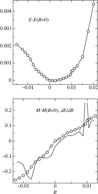
Magnetization and total energy (relative to the B=0 case) were generated for several values of B, and ∂E/∂B was obtained from numerical differentiation of E.
As the top figure shows, the total energy E has a minimum near, but not exactly at B=0. This shows that there are some slight errors in the LDA calculation (in an exact self-consistent LDA calculation E should be minimum at exactly B=0). E is smooth in the interval (−0.01, 0.01) Ry, as the figure shows. The behavior is somewhat unsmooth near B=−0.01 Ry, and its discontinuity or near discontinuity is evident near B=0.01 Ry. That means numerical differentiation ∂E/∂B is a bit problematic, particularly outside the (−0.01,0.01) interval. Nevertheless we can perform it. In the bottom figure, M−M(B=0) and ∂E/∂B are plotted respectively as a function of B as dashed lines+circles, and a solid line. The two curves track fairly well, though ∂E/∂B is noisy; nor is M(B) particularly smooth.
We can obtain χ from the slope ∂E/∂B. There is some uncertainty in the calculation since M is not particularly smooth (note in particular that (∂E/∂B)+ and (∂E/∂B)− are a little different).
We can also obtain both χ0 by obtaining δM0 from a 1-shot calculation. The table below shows M0 and M for two values of B:
| B | M0 | M |
|---|---|---|
| -0.005 | -2.363587 | -2.402973 |
| 0.005 | -2.234213 | -2.219662 |
Thus we get:
As noted above, I calculated in this way only approximately corresponds to the Stoner I. A better calculation should produce I about 1 eV.