CTQMC for NiO
Running the DMFT loop
Introduction
You have all the input files here this link. Untar it to access all the files and copy them into a directory where you want to run the DMFT calculations; let’s call it dmftrun again.
Running the loop
The DMFT loop is composed by alternated runs of lmfdmft and ctqmc, the output of each run being the input for the successive. To do that, do the following steps:
1. Prepare and launch the lmfdmft run
We are using the hybridization expansion CT-QMC solver. So before launching the solver we need to prepare the hybridization matrix for the Ni 3-d correlated orbitals. But now we got two Ni atoms as correlated atoms in the unit cell and the indmfl file needs to be accordingly modified. The switches here are special and meant for an antiferromagnetic calculation that copies the self energy of one correlated atom after spin flipping to the other correlated atom, so that the net moment on both correlated blocks is zero. The indmfl.nio looks like:
0.1 1.2 1 2                # hybridization Emin and Emax, measured from FS, renormalize for interstitials, projection type
1 0.0025 0.0025 600 -3.000000 1.000000  # matsubara, broadening-corr, broadening-noncorr, nomega, omega_min, omega_max (in eV)
2                                     # number of correlated atoms
1     1   0                           # iatom, nL, locrot
  2   2   1                           # L, qsplit, cix
2     1   0                           # iatom, nL, locrot
  2   2  -1                           # L, qsplit, cix
#================ # Siginds and crystal-field transformations for correlated orbitals ================
1     5   5       # Number of independent kcix blocks, max dimension, max num-independent-components
1     5   5       # cix-num, dimension, num-independent-components
#---------------- # Independent components are --------------
'x^2-y^2' 'z^2' 'xz' 'yz' 'xy'
#---------------- # Sigind follows --------------------------
1 0 0 0 0
0 2 0 0 0
0 0 3 0 0
0 0 0 4 0
0 0 0 0 5
#---------------- # Transformation matrix follows -----------
 0.70710679 0.00000000   0.00000000 0.00000000   0.00000000 0.00000000   0.00000000 0.00000000   0.70710679 0.00000000
 0.00000000 0.00000000   0.00000000 0.00000000   1.00000000 0.00000000   0.00000000 0.00000000   0.00000000 0.00000000
 0.00000000 0.00000000   0.70710679 0.00000000   0.00000000 0.00000000  -0.70710679 0.00000000   0.00000000 0.00000000
 0.00000000 0.00000000   0.00000000 0.70710679   0.00000000 0.00000000   0.00000000 0.70710679   0.00000000 0.00000000
-0.70710679 0.00000000   0.00000000 0.00000000   0.00000000 0.00000000   0.00000000 0.00000000   0.70710679 0.00000000
2     5   5       # cix-num, dimension, num-independent-components
#---------------- # Independent components are --------------
'x^2-y^2' 'z^2' 'xz' 'yz' 'xy'
#---------------- # Sigind follows --------------------------
6 0 0 0 0
0 7 0 0 0
0 0 8 0 0
0 0 0 9 0
0 0 0 0 10
#---------------- # Transformation matrix follows -----------
 0.70710679 0.00000000   0.00000000 0.00000000   0.00000000 0.00000000   0.00000000 0.00000000   0.70710679 0.00000000
 0.00000000 0.00000000   0.00000000 0.00000000   1.00000000 0.00000000   0.00000000 0.00000000   0.00000000 0.00000000
 0.00000000 0.00000000   0.70710679 0.00000000   0.00000000 0.00000000  -0.70710679 0.00000000   0.00000000 0.00000000
 0.00000000 0.00000000   0.00000000 0.70710679   0.00000000 0.00000000   0.00000000 0.70710679   0.00000000 0.00000000
-0.70710679 0.00000000   0.00000000 0.00000000   0.00000000 0.00000000   0.00000000 0.00000000   0.70710679 0.00000000
You can now find the DMFT tag, temperature at which CT-QMC should be performed, number of matsubara frequencies, and the choice of the projection window in the tag right at the bottom of the ctrl.nio file. It reads like:
DMFT PROJ=2 NLOHI=11,26 BETA=50 NOMEGA=999 KNORM=0
So, as before, we have to run_lmfdmft_{:.exec} twice to start with; first to prepare a sig.inp with all zeroes and then to prepare the hybridization matrix (delta.ni) and chemical potentials (eimp1.ni).
cd dmftrun
mpirun -n 24 lmfdmft -vnkabc=8 --rs=1,0 --ldadc=28.95 -job=1 ctrl.nio
mpirun -n 24 lmfdmft -vnkabc=8 --rs=1,0 --ldadc=28.95 -job=1 ctrl.nio
This would take around 40 seconds to complete the job and produce the hybridization matrix (delta.ni) and chemical potentials (eimp1.ni) for the correlated impurity states. There are 5 d-orbitals and two spins, so the delta.ni file has 21 columns in total and is written in the same format as sig.inp. eimp1.ni file has information about the energies of the impurity levels.
Now we need to rename few files and edit some files to make sure the solver reads what it looks for. Also the PARAMS file that knows about all the parameters for CT-QMC and DMFT should read the energies for the impurity levels and chemical potential from the recently created eimpi.ni file:
cp delta.nio Delta.inp
cp eimp1.nio Eimp.inp
echo "Ed [ -34.145881, -34.144891, -34.319678, -34.145306, -34.303933, -32.748547, -32.748459, -26.563071, -32.748503, -26.561103]" >> PARAMS                         # identify the impurity levels inside the PARAMS file
echo "mu   34.145881" >> PARAMS                           # identify the starting chemical potential inside the PARAMS file
At this point the PARAMS file should look like this
OffDiagonal  real
Sig  Sig.out
Gf  Gf.out
Delta  Delta.inp
cix  actqmc.cix
mode GM
Nmax  600         # Maximum perturbation order allowed
nom  120          # Number of Matsubara frequency points sampled
exe  ctqmc        # Name of the executable
tsample  20       # How often to record measurements
Ed [ -34.145881, -34.144891, -34.319678, -34.145306, -34.303933, -32.748547, -32.748459, -26.563071, -32.748503, -26.561103] # Ed: Eimp-Edc for PARAMS
M  80000000       # Total number of Monte Carlo steps per core
Ncout  5000000            # How often to print out info
PChangeOrder  0.9         # Ratio between trial steps: add-remove-a-kink / move-a-kink
mu   34.145881 # mu = -Eimp[0] for PARAMS
warmup  5000000           # Warmup number of QMC steps
sderiv  0.02      # Maximum derivative mismatch accepted for tail concatenation
aom  10           # Number of frequency points used to determin the value of sigma at nom
U    4.0
J    0.3
nf0  8.0
beta 50.0
The PARAMS file is self explanatory. However we should be careful while choosing numbers for U, J, n and and make sure they are consistent with the choice of our double counting correction (ldadc) and the information inside the ctrl.ni file. Once the PARAMS file is ready we can now run a script called atom_d.py, which will generate all the essential information about the Hilbert space for the correlated impurity. But before that we also should have the file called Trans.dat in the path which knows about the size of the correlated block and the transformation matrix that connects the real harmonics to the spherical Harmonics for the correlated d-orbitals. For Nickel it looks similar to what is shown below, where the block containing numbers from 1 to 5 stands for one kind of spin and 6 to 10 for the other kind.
  10 10 #  size of Sigind and CF
#---- Sigind follows
  1    0    0    0    0    0    0    0    0    0
  0    2    0    0    0    0    0    0    0    0
  0    0    3    0    0    0    0    0    0    0
  0    0    0    4    0    0    0    0    0    0
  0    0    0    0    5    0    0    0    0    0
  0    0    0    0    0    6    0    0    0    0
  0    0    0    0    0    0    7    0    0    0
  0    0    0    0    0    0    0    8    0    0
  0    0    0    0    0    0    0    0    9    0
  0    0    0    0    0    0    0    0    0   10
#---- CF follows
  0.00000000  0.70710679   0.00000000  0.00000000   0.00000000  0.00000000   0.00000000  0.00000000   0.00000000 -0.70710679   0.00000000  0.00000000   0.00000000  0.00000000   0.00000000  0.00000000   0.00000000  0.00000000   0.00000000  0.00000000
  0.00000000  0.00000000   0.00000000  0.70710679   0.00000000  0.00000000   0.00000000  0.70710679   0.00000000  0.00000000   0.00000000  0.00000000   0.00000000  0.00000000   0.00000000  0.00000000   0.00000000  0.00000000   0.00000000  0.00000000
  0.00000000  0.00000000   0.00000000  0.00000000   1.00000000  0.00000000   0.00000000  0.00000000   0.00000000  0.00000000   0.00000000  0.00000000   0.00000000  0.00000000   0.00000000  0.00000000   0.00000000  0.00000000   0.00000000  0.00000000
  0.00000000  0.00000000   0.70710679  0.00000000   0.00000000  0.00000000  -0.70710679  0.00000000   0.00000000  0.00000000   0.00000000  0.00000000   0.00000000  0.00000000   0.00000000  0.00000000   0.00000000  0.00000000   0.00000000  0.00000000
  0.70710679  0.00000000   0.00000000  0.00000000   0.00000000  0.00000000   0.00000000  0.00000000   0.70710679  0.00000000   0.00000000  0.00000000   0.00000000  0.00000000   0.00000000  0.00000000   0.00000000  0.00000000   0.00000000  0.00000000
  0.00000000  0.00000000   0.00000000  0.00000000   0.00000000  0.00000000   0.00000000  0.00000000   0.00000000  0.00000000   0.00000000  0.70710679   0.00000000  0.00000000   0.00000000  0.00000000   0.00000000  0.00000000   0.00000000 -0.70710679
  0.00000000  0.00000000   0.00000000  0.00000000   0.00000000  0.00000000   0.00000000  0.00000000   0.00000000  0.00000000   0.00000000  0.00000000   0.00000000  0.70710679   0.00000000  0.00000000   0.00000000  0.70710679   0.00000000  0.00000000
  0.00000000  0.00000000   0.00000000  0.00000000   0.00000000  0.00000000   0.00000000  0.00000000   0.00000000  0.00000000   0.00000000  0.00000000   0.00000000  0.00000000   1.00000000  0.00000000   0.00000000  0.00000000   0.00000000  0.00000000
  0.00000000  0.00000000   0.00000000  0.00000000   0.00000000  0.00000000   0.00000000  0.00000000   0.00000000  0.00000000   0.00000000  0.00000000   0.70710679  0.00000000   0.00000000  0.00000000  -0.70710679  0.00000000   0.00000000  0.00000000
  0.00000000  0.00000000   0.00000000  0.00000000   0.00000000  0.00000000   0.00000000  0.00000000   0.00000000  0.00000000   0.70710679  0.00000000   0.00000000  0.00000000   0.00000000  0.00000000   0.00000000  0.00000000   0.70710679  0.00000000
Run atom_d.py using the command
atom_d.py J=0.3 l=2 OCA_G=False "CoulombF='Ising'" "Eimp=[ 0.000000, 0.000990, -0.173797, 0.000575, -0.158052, 1.397333, 1.397422, 7.582810, 1.397378, 7.584777]"where the argument Eimp is a copy of the third line of Eimp.inp (to be changed at each iteration accordingly to the previous lmfdmft run) and the argument J is the Hund’s coupling.
l=2means the correlated impurity contains d-electrons. If the correlated impurity contains f-electrons (say for elemental Cerium) thenlshould be changed to 3. OCA_G=False implies that we don’t want to use One Crossing Approximation (OCA) as the impurity solver.CoulombF='Ising'implies that the interaction matrix is density-density. Alternatively, we can useCoulombF='Full'to work with a full slater-inetraction matrix for the correlated impurity.Running atom_d.py generates two files; actqmc.cix and info_atom_d.py used by the ctqmc solver. Now, let’s launch the CT-QMC solver.
mpirun -n 24 ctqmc
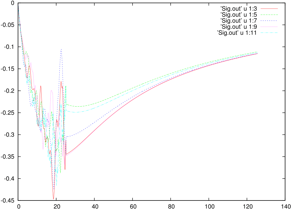
The imaginary part of the self energy would look ugly and something like this:
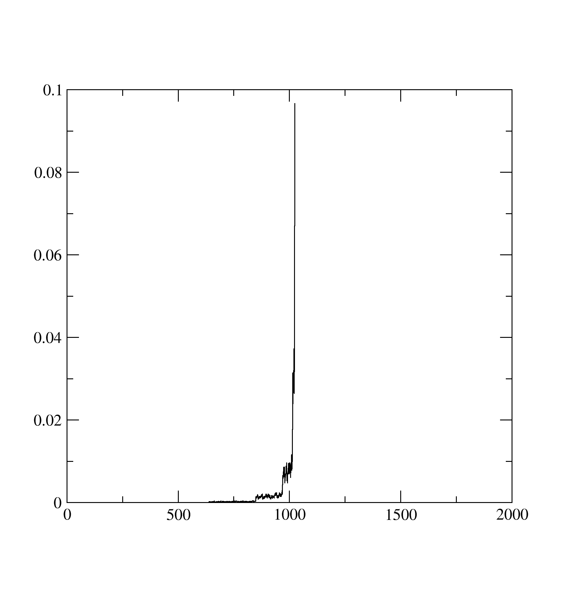
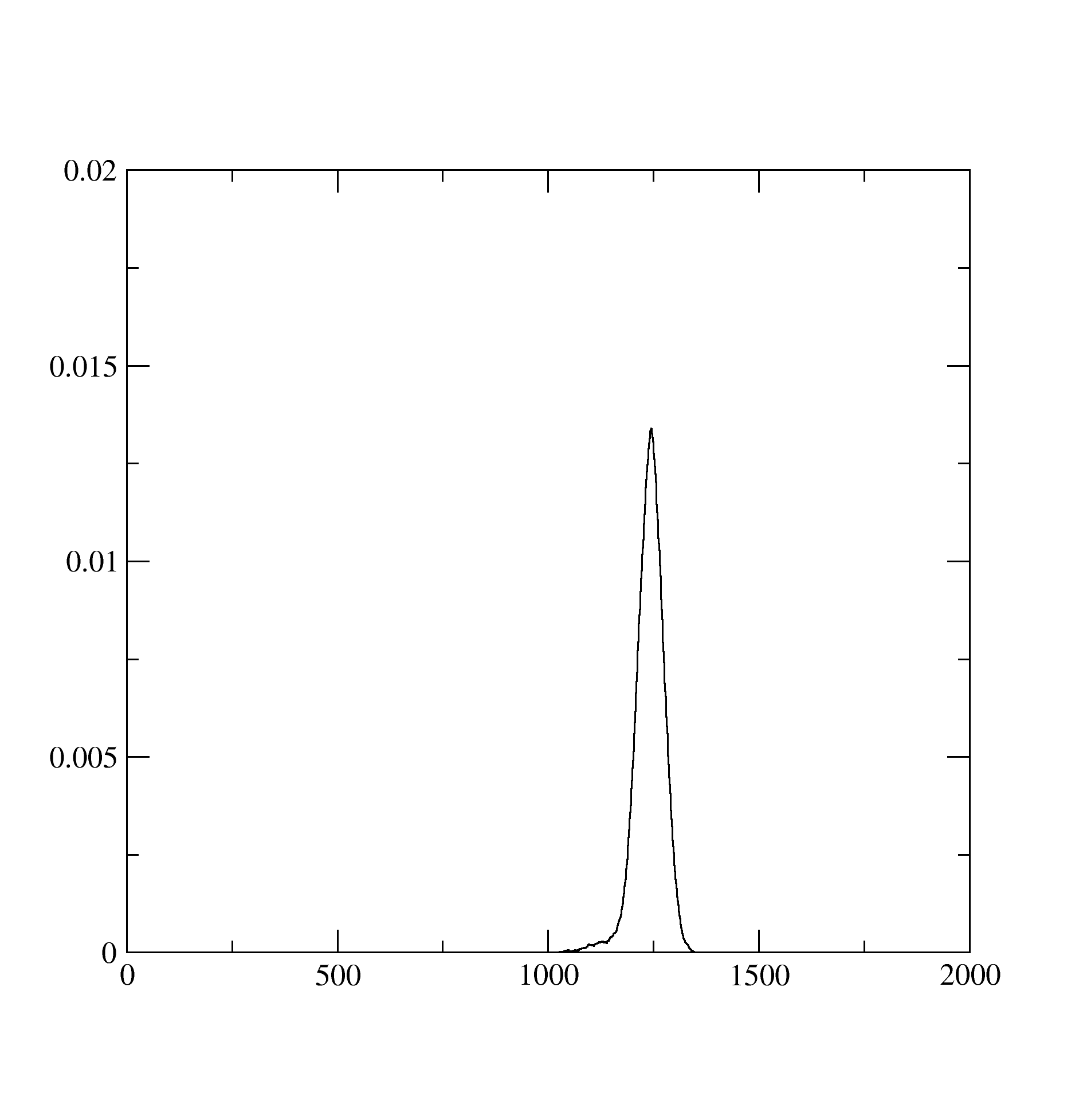
The histogram.dat stores information about the expnasion orders in hybridization that contributed dominantly to the solution. It looks like below and suggests that at least the expansion upto 1200 th order contributed:
The Probability.dat stores the information about probabilities of occurence of different atomic states: