Nb/Fe/Nb Metallic Trilayer, Electronic Structure and Landauer-Buttiker Transport
This tutorial studies the Landauer-Buttiker transport through a Nb/Fe/Nb trilayer. The setup of the trilayer is complicated, and as a first step the Nb/Fe superlattice (with periodic boundary conditions) is constructed, as explained in this tutorial. There is also a related tutorial on the Nb/Ni/Nb trilayer.
Nb and Fe are both bcc but are strongly lattice mismatched, and it necessitated rotating them to axes different from the cubic axes. See the Nb/Fe superlattice tutorial for its construction and the relaxation of atoms at the interface.
This tutorial begins where the superlattice tutorial leaves off. It uses the Atomic Spheres Approximation, and the principal layer code designed to calculate Landauer-Buttiker transmission through a multilayer.
There is an additional complication when the ASA is used — namely sphere packing for overlapping spheres becomes a challenge for a complex interface such as this. The early parts of this tutorial modify the original SL by adding empty spheres, before proceeding to the (nonperiodic) Nb/Fe/Nb trilayer.
Table of Contents
- Preliminaries
- Introduction and Basic Strategy
- 1. Self-consistent ASA-LDA energy bands for reconstructed Nb
- 2. Self-consistent ASA-LDA energy bands for reconstructed Fe
- 3. ASA Structure file for the Nb/Fe superlattice
- 4. Self-Consistent ASA calculation of the Nb/Fe superlattice
- 5. Crystal Green’s function calculation of the Nb/Fe superlattice
- 6. Nb/Fe/Nb Trilayer
- Appendix. ASA restart file editor instructions
- Footnotes and references
Section 1. Energy bands of Nb (3×1) reconstructed cell in the ASA
Requires files init.nb and site3.nb. Creates files rsta.nbasa and fplot.ps
cp init.nb init.nbasa
blm --gf --nl=3 --nfile --nk=12,12,12 --asa nbasa
cat actrl.nbasa | sed 's/LMX=2/LMX=2  GRP2=1/'  | awk '{ if ($1 == "OPTIONS") {print "HAM   PMIN=-1 QASA=1"}; print}' > ctrl.nbasa
cp site3.nb site3.nbasa
lmstr -vfile=3 ctrl.nbasa
touch nb.nbasa; rm -f nb*.nbasa
lm -vnit=0 -vfile=3 ctrl.nbasa
lm -vnit=30 -vfile=3 ctrl.nbasa --rs=0,1
mcx -cmpf:fn1=rsta.nbasa:fn2=`echo ~/lmf/testing/nbfe/rsta.nbasa`
lmchk ctrl.nbasa -vfile=3 --syml~n=31~q=0,1,0,0,0,0,1/2,0,-1/2
lm -vnit=30 -vfile=3 ctrl.nbasa --band~fn=syml
echo -6,6,5,10 | plbnds -fplot~sh~scl=.5 -ef=0 -scl=13.6 --nocol -dat=red nbasa
fplot -f plot.plbnds
open fplot.ps
Self -consistent lmgf:
cp ~/lmf/testing/nbfe/rsta.nbasa rsta.nbasa
rm -f save.nbasa mixm.nbasa sv.nbasa log.nbasa vshft.nbasa
lmgf -vnit=0 -vfile=3 ctrl.nbasa --rs=1,0
lmgf ctrl.nbasa -vfile=3 -vccor=f -vnit=1 --pr40,21 -vgamma=t --quit=rho
rm -f save.nbasa mixm.nbasa sv.nbasa log.nbasa
lmgf ctrl.nbasa -vfile=3 -vccor=f -vnit=50 --pr40,21 -vgamma=t
mcx -cmpf:fn1=save.nbasa:fn2=`echo ~/lmf/testing/nbfe/save.nbasa.gf`
Section 2. Energy bands of Fe (4×1) reconstructed cell in the ASA Requires files init.fe and site4.fe. Creates files rsta.feasa and fplot.ps
cp init.fe init.feasa
blm --nfile --nk=10,5,13 --mag --asa feasa
cat actrl.feasa | sed 's/\(MMOM.*\)/\1 GRP2=1/'  | awk '{ if ($1 == "OPTIONS") {print "HAM   PMIN=-1 QASA=1"}; print}' > ctrl.feasa
cp site4.fe site4.feasa
lmstr -vfile=4 ctrl.feasa
lm -vnit=0 -vfile=4 ctrl.feasa
lm -vnit=30 -vfile=4 ctrl.feasa --rs=0,1
cp syml.nbasa syml.feasa
lm -vnit=30 -vfile=4 ctrl.feasa --band~fn=syml
echo -6,6,5,10 | plbnds -fplot~sh~scl=.5 -ef=0 -scl=13.6 --nocol -dat=red -spin1 feasa
fplot -f plot.plbnds
open fplot.ps
Section 3. ASA Structure file for the Nb/Fe superlattice
Requires file site4.nbfe. This file is generated in the full-potential tutorial for Nb/Fe superlattices. Generate it using that tutorial, or if you want to proceed directly without working through that tutorial, you can use ~/lmf/testing/nbfe/site9.asa.
A condensed version of the commands in Section 3 have been bundled into a script, ~/lmf/testing/test.nbfeasa. For quick execution of Section 3, run this script
~/lmf/testing/test.nbfeasa 1
It does the following:
a. Use blm to make temporary ctrl file from site9.asa (output = ctrl)
b. Use lmscell to relabel Nb and Fe sites at the Nb/Fe interface, rendering them inequivalent (output = site8)
c. Use blm to make a new ctrl file with additional species, and site file with empty spheres (output = site7)
d. Use sed to modify ctrl.asa, constraining the MT radius of bulk Nb to that of the value in elemental Nb, and create a SPEC category with ES radii adjusted to file spacing (output = spec)
e. Use blm to remake the ctrl file from new SPEC and site data
f. Use lmchk to optimally place ES (output = site6)
g. Use lmscell to reorder site positions with increasing projection along normal plane (output = site5)
Section 4. Self-Consistent ASA calculation of the Nb/Fe superlattice
This section requires files site5.asa and rsta.nbasa and rsta.feasa. These files are generated in Sections 3, 1, and 2 respectively. If you want to proceed directly without working through those parts, you can find them in ~/lmf/testing/nbfe.
A condensed version of the commands in Section 4 have been bundled into ~/lmf/testing/test.nbfeasa. For quick execution of Section 3, do the following.
Trial density:
~/lmf/testing/test.nbfeasa 1 2
Job 2 uses lm with –rsedit to create an initial density; copies rsta files for bulk Nb and Fe into files rsta2 and rsta3. Output is rsta.asa.
Self-consistent density with band code lm.
~/lmf/testing/test.nbfeasa [--MPIK] 3
Job 3 does the following:
a. Runs lm with scr=11 to make the static ASA response function (output = psta)
b. Runs lm using scr=2 to converge to self-consistency (output = rsta5)
Note: To run test.nbfeasa 3, you must precede it by jobs 1 and 2. You can do, e.g.
~/lmf/testing/test.nbfeasa 1 2 3
Energy bands
lmchk ctrl.asa  --syml~n=41~q=0,1,0,0,0,0,1,0,-1
lm -vmet=3 ctrl.asa -vccor=f -vnit=1 --pr40,21 --quit=rho --band~col=1:134,243:360~col2=135:242~fn=syml
echo -5,5,5,10 | plbnds -spin1 -fplot~sh~scl=.7~shft=-.28 -ef=0 -scl=13.6 -dat=up -lt=1,col=0,0,0,colw=1,0,0,colw2=0,1,0 bnds.asa
open fplot.ps
echo -5,5,5,10 | plbnds -spin2 -fplot~sh~scl=.7~shft=.45 -ef=0 -scl=13.6 -dat=dn -lt=1,col=0,0,0,colw=1,0,0,colw2=0,1,0 bnds.asa
open fplot.ps
Section 5. Self-Consistent ASA Green’s function calculation of the Nb/Fe superlattice
This section should follow the preceding ones. To run it standalone, the following setup should be sufficient:
~/lmf/testing/test.nbfeasa --quiet 1 2
lmstr asa
cp ~/lmf/testing/nbfe/rsta.asa.lm .
Then do:
~/lmf/testing/test.nbfeasa [--MPIK] 4
It does the following:
a. Runs lm with scr=11 to make the static ASA response function (output = psta)
b. Runs lmgf using scr=2 to converge to self-consistency
The script creates a compact restart file rsta.asa.lmgf with the self-consistent density, and vshft.asa.gf with the potential shifts.
Section 6. The Nb/Fe/Nb Trilayer
Steps in section should follow section 5. You cannot run it standalone. Steps are bundled into test.nbfeasa :
~/lmf/testing/test.nbfeasa [--MPIK] 5
Job 5 does the following:
a. Uses blm to add PGF category to the ctrl file and also set LMX=2 (output = ctrl) XX
b. Uses lmscell to assign principal layers (site4)
c. Runs lm with scr=11 to make the static ASA response function in this basis (output = psta)
d. Runs lmgf using scr=2 to converge to self-consistency in larger basis
e. Uses lmpg –rsedita to create a starting potential into a trilayer form suitable for lmpg, importing rsta for basis sites from lmgf and rsta for padding layers from bulk Nb f. Makes L- and R- end leads self-consistent
g. Makes the active region self-consistent (output = rsta.asa.lmgf)
Preliminaries
The tutorial has several Sections. Intermediate sections may be skipped: you can start the tutorial at any of Sections 1,2,3,4, provided you copy the necessary starting files from your Questaal source directory (where you cloned the Questaal package). For purposes of this tutorial we will assume it is ~/lmf. A condensed form of the entire tutorial has been bundled into a standard test case. You can invoke ~/lmf/testing/test.nbfeasa from any empty directory and let the script perform the steps for you. It’s an easy way to see what you should get, if you have problems.
This tutorial makes extensive use of many of the Questaal packages. including lmscell, lmplan, lm, lmgf, lmpg, and miscellaneous utilities such as vextract. They are assumed to be in your path.
Questaal invokes mpix to execute MPI jobs. mpix is a proxy for mpirun, the default command that launches MPI jobs. We assume your system has 16 processors on a core, but you can use any number, or run in serial.
For drawing postscript files, this tutorial assumes you will use the Apple open. Substitute your postscript viewer of choice for open.
Required Input files
This tutorial uses the following files from Nb/Fe superlattice tutorial init.nb, site3.nb, init.fe, site4.fe all found in this section, and site4.nbfe, created in this section. If you want to skip that tutorial, you can
Copy file init.nb to init.nbasa:
# Init file for Nb.  Lattice constant at 0K
LATTICE
    ALAT=6.226 PLAT= -.5 .5 .5  .5 -.5 .5  .5 .5 -.5
SPEC ATOM=Nb  PZ=0,0,0
SITE
    ATOM=Nb   X=0 0 0
File site3.nb
% site-data vn=3.0 fast io=31 nbas=3 alat=6.226 plat= -0.5 0.5 0.5 1.5 1.5 -1.5 0.0 0.0 1.0
#                        pos
 Nb        0.0000000   0.0000000   0.0000000
 Nb        0.5000000   0.5000000  -0.5000000
 Nb        1.0000000   1.0000000  -1.0000000
File init.fe
# Init file for Fe.  Lattice constant at 0K
LATTICE
    ALAT=5.404 PLAT= -.5 .5 .5  .5 -.5 .5  .5 .5 -.5
SPEC
    ATOM=Fe  MMOM=0,0,2.2
SITE
    ATOM=Fe   X=0 0 0
File site4.fe
% site-data vn=3.0 fast io=15 nbas=4 alat=6.226 plat= -0.5 0.5 0.5 1.5 1.5 -1.5 0.18425022 -0.50338096 0.68763117
#                        pos
 Fe        0.0000000   0.0000000   0.0000000
 Fe        0.0000000   0.7500000   0.0000000
 Fe        0.5000000   1.0000000  -0.5000000
 Fe        1.0000000   1.2500000  -1.0000000
Introduction and Basic Strategy
This tutorial shows how to make a self-consistent density starting from the superlattice developed in the Nb/Fe superlattice tutorial, within the Atomic Spheres approximation.
Initially the ASA-LDA code lm code is then applied to the relaxed superlattice to confirm the reliability of the ASA.
Next the crystal Green’s function package lmgf as setup to the layer Green’s function package lmpg.
Finally a structure is set up for trilayer geometry (… Nb / Fe / Nb …), which is related to but distinct from the Nb/Fe superlattice, as it is not periodic along the stacking axis. Transmission calculations through the trilayer are performed using lmpg.
In the Nb/Fe superlattice tutorial a superlattice of Nb and Fe was constructed; structural information is contained in site4.nbfe. Starting from it this tutorial will do:
- Make a ctrl and site file suitable for the ASA, with periodic boundary conditions. The interface has an additional complication in that open spaces appear, which the ASA must deal with by packing with additional empty spheres. Care must be taken to fill space, but not allow the sphere overlaps become too large.
- Repeat the self-consistent calculation of the interface code with the ASA-LDA code lm. lm is more approximate than the full LDA code lmf, but it is very efficient, and provides a stepping stone to final objective, transport through a trilayer
- Repeat the calculation once again with the crystal Green’s function code, lmgf, and demonstrate that the spectral functions are similar to the bands created by lm.
- Setup the trilayer geometry.
- Calculate transmission with the transport code, lmpg.
1. Self-consistent ASA-LDA energy bands for reconstructed Nb
It is instructive to perform a band calculation for Nb in the (3×1) reconstructed superlattice in the ASA approximation, to compare it to the full LDA result generated here.
This step isn’t essential for the superlattice, but it is useful as a sanity check we will need the ASA for transport and need to confirm its reliability for bulk Nb.
cp init.nb init.nbasa
blm --nl=3 --nfile --nk=12,12,12 --asa nbasa
cat actrl.nbasa | sed 's/LMX=2/LMX=2  GRP2=1/'  | awk '{ if ($1 == "OPTIONS") {print "HAM   PMIN=-1 QASA=1"}; print}' > ctrl.nbasa
blm makes an acceptable ctrl file, but we make a few tweaks in anticipation of the fact that ultimately we will use lmpg for transport. This code doesn’t allow down-folding, and it uses KKR style accumulation of weights. Compare the changes and refer to the input file documentation for the meaning of each new tag.
Check the sphere overlaps
cp site3.nb site3.nbasa
lmchk -vfile=3 ctrl.nbasa --shell
Because of the reconstruction, the three Nb split into two classes. Each class has 8 nearest neighbors, 6 second neighbors, 12 third neighbors, etc. characteristic of the bcc latttice. The MT sphere has been enlarged relative to the full-potential result so that the sphere volume matches the unit cell volume, as the ASA requires (look for Sum of sphere volumes).
Make the ASA density self-consistent in the reconstructed structure, storing moments in rsta.nbasa
lmstr -vfile=3 ctrl.nbasa
lm -vnit=0 -vfile=3 ctrl.nbasa
lm -vnit=30 -vfile=3 ctrl.nbasa --rs=0,1
To check that the code executed correctly, compare against the reference:
mcx -cmpf:fn1=rsta.nbasa:fn2=`echo ~/lmf/testing/nbfe/rsta.nbasa`
The maximum difference should be small (of order 10−5 or less)
Draw the ASA bands:
lmchk ctrl.nbasa -vfile=3 --syml~n=31~q=0,1,0,0,0,0,1/2,0,-1/2
lm -vnit=30 -vfile=3 ctrl.nbasa --band~fn=syml
echo -6,6,5,10 | plbnds -fplot~sh~scl=.5 -ef=0 -scl=13.6 --nocol -dat=red nbasa
fplot -f plot.plbnds
open fplot.ps
The ASA energy bands are quite similar to the full LDA ones, and sufficiently close for the present purposes. Note the bands cross the Fermi surface at similar points with similar slope.

Blue: LDA bands generated by lmf. Red: ASA-LDA generated by lm.
ASA Green’s function for reconstructed Nb
The ASA suite also has a crystal Green’s function code, lmgf. This page has a basic tutorial describing lmgf and its operation. lmgf is of particular interest here mainly as a segue into the principal layer Green’s function code, lmpg.
lmgf operates in a manner approximately similar to lm but it generates Green’s functions instead of wave functions. lmgf reads the same potential parameters as lm but constructs the Green’s function instead of a hamiltonian. The program flow is similar to lm, only the “crystal” branch is replaced by a branch that obtains multipole moments through Green’s functions. Multipole moments provide a compact way to represent the charge density in the ASA: the ability to generate them enables lmgf to perform self-consistent calculations.
If the Hamiltonian lm and lmgf were identical, they should produce identical charge densities. This is only approximately true: the third order parameterization of the potential function P are not identical; see Sec 2.13.4. in Ref. 1 for details.
As noted in the Introductory tutorial, lmgf requires some additional input, namely a GF category and an EMESH tag in the BZ category. It is strongly advised that you run through that tutorial before doing this section.
The elliptical energy contour, normally used for Brillouin zone integrations needed, e.g. to find the Fermi level and the output moments, requires information about the Fermi level. It is easiest to get an estimate from lm, since the two methods are closely linked. From the last output of lm, the Fermi level is displayed in a table with a line
 BZINTS: Fermi energy:     -0.011371;  15.000000 electrons;  D(Ef):   54.706
 ...
The Fermi level appropriate to lmgf should be close to −0.01 Ry, but not identically so because lmgf uses a different integration scheme and the third order Green’s function is close to, but identical with the 3rd order ASA hamiltonian.
Run lmgf to get the Fermi level satisfying charge neutrality. This is a nonlinear problem, so EF must be found iteratively (see also the Introductory tutorial). Here we choose EF to be zero (specified in the input file) but add a constant potential shift in the entire system to satisfy charge neutrality.
This should not be necessary, but to synchronize exactly with the tutorial, update the starting potential from the reference rsta file:
cp ~/lmf/testing/nbfe/rsta.nbasa rsta.nbasa
lmgf -vnit=0 -vfile=3 ctrl.nbasa --rs=1,0
Then do:
rm -f save.nbasa mixm.nbasa sv.nbasa log.nbasa vshft.nbasa
lmgf ctrl.nbasa -vfile=3 -vccor=f -vnit=1 --pr40,21 -vgamma=t --quit=rho
–quit=rho tells lmgf to stop after vconst has been found. The output should show a series of tables, the first being:
 GFASA:  integrated quantities to efermi = 0
 ...
         deviation from charge neutrality: 0.744264
This shows that EF needs to be shifted to accommodate 0.74 electrons. It uses a fast method (a Pade approximation to ) to find an estimate for the shift. It iterates the Pade approximation until charge neutrality is found. It settles on a converged value
 gfasa:  potential shift this iter = 0.018645.  Cumulative shift = 0.018645
 shift (0.019) within Pade tolerance (0.03, tolq=0) ... accept Pade correction to G
The shift was small enough to fit within the specified Pade tolerance 0.03 (0.03 is a default tolerance, which is used unless you specify padtol=# in GFOPTS). Had the shift been too large for the Pade to be reliable, lmgf will remake the full in the presence of the shifted potential. It will continue to do this until The Pade correction falls below the tolerance.
The RMS DQ is printed in this line:
PQMIX: read 0 iter from file mixm. RMS DQ=4.61e-3
It is small enough that further self-consistency is not really necessary (self-consistent potential generated by lm and lmgf are very similar). Neverthess we can make it self-consistent:
rm -f save.nbasa mixm.nbasa sv.nbasa log.nbasa
lmgf ctrl.nbasa -vfile=3 -vccor=f -vnit=50 --pr40,21 -vgamma=t
It should converge smoothly in 7 iterations, with a converged potential shift vconst=0.0203157 (file vshft.nbasa).
lmchk ctrl.nbasa -vfile=3 --syml~n=101~q=0,1,0,0,0,0,1/2,0,-1/2
lmgf ctrl.nbasa -vnz=501 -vnsp=2 -vfile=3 -vccor=f -vnit=50 --pr40,21 -vgamma=t --band:fn=syml --quit=rho
SpectralFunction.sh  -w -5:2
open asa_UP.png
open asa_DN.png
2. Self-consistent ASA-LDA energy bands for reconstructed Fe
As in the Nb case, it is instructive to perform a band calculation for ferromagnetic Fe in the (4×1) reconstructed superlattice in the ASA approximation, to compare it to the full LDA result generated here.
cp init.fe init.feasa
blm --nfile --nk=10,5,13 --mag --asa feasa
cat actrl.feasa | sed 's/\(MMOM.*\)/\1 GRP2=1/'  | awk '{ if ($1 == "OPTIONS") {print "HAM   PMIN=-1 QASA=1"}; print}' > ctrl.feasa
Check the sphere overlaps
cp site4.fe site4.feasa
lmchk -vfile=4 ctrl.feasa
The MT sphere has been enlarged so that the sphere volume matches the unit cell volume, as the ASA requires.
Make the ASA density self-consistent in the reconstructed structure, storing moments in rsta.feasa
lmstr -vfile=4 ctrl.feasa
lm -vnit=0 -vfile=4 ctrl.feasa
lm -vnit=30 -vfile=4 ctrl.feasa --rs=0,1
Draw the ASA bands:
cp syml.nbasa syml.feasa
lm -vnit=30 -vfile=4 ctrl.feasa --band~fn=syml
echo -6,6,5,10 | plbnds -fplot~sh~scl=.5 -ef=0 -scl=13.6 --nocol -dat=red -spin1 feasa
open fplot.ps
echo -6,6,5,10 | plbnds -fplot~sh~scl=.5 -ef=0 -scl=13.6 --nocol -dat=red -spin2 feasa
open fplot.ps
As with Nb, the ASA energy bands are quite similar to the full LDA ones, and indeed significantly closer to each other than to bands computed from a higher level theory such as GW.
Majority (left) and minority (right) energy bands of Fe. blue: LDA generated by lmf; red: ASA-LDA generated by lm.

3. ASA Structure file for the Nb/Fe superlattice
The ASA is more difficult to set up because of the constraint that the spheres fill space: the sum-of-sphere volumes must equal the volume of the unit cell. Also In the end regions we want to keep the spheres the same as the bulk Nb. At the interface there is considerable reconstruction which makes good sphere packing difficult.
We require the structure generated by the Nb/Fe superlattice tutorial. If you did that tutorial, copy the structure file of the relaxed interface, site4.nbfe, to file site9.asa to your working directory.
Alternatively you can begin immediately starting with Section 3 by doing the following:
touch site9.asa; rm -f *.asa ; cp /h/ms4/lmf/b/./testing/nbfe/{site9.asa,rsta.nbasa,rsta.feasa} .
Note: a script has been written to perform all these steps automatically (part of the standard Questaal tests). The steps are a bit involved, and the script is useful as a sanity check to check that you’ve done all the steps in the proper order. To perform all the steps of this section automatically, do the following:
~/lmf/testing/test.nbfeasa --quiet 1
A working ctrl file is needed to use Questaal’s tools. The ctrl file in the Nb/Fe superlattice tutorial was designed for lmf, and it is a bit different from the ASA.
We make an temporary ctrl file, taking minimum information from that tutorial and build ctrl.asa from scratch. Make a preliminary file with
blm --nfile --rdsite=site9 --nosort --shorten=no --ctrl=ctrl asa
To manage sphere packing in the ASA we must distinguish sites immediately at the interface from those in the bulk. Recall the superlattice geometry:
  Layer    Nb 1      Nb 2      Fe 1       Fe 2     Fe 3      Nb 3      Nb 4
  sites    1-3       4-6       7-10       11-14    15-18     19-21     22-24
The frontier sites are 4-6 and 19-21 (Nb) and 7-10 and 15-18 (Fe). Use the lmscell, utility to assign species Nbx and Fex to these files, or alternatively just use a text editor and do it by hand. The following creates site8.asa
lmscell ctrl.asa --stack~setlbl@spid=Nbx@targ=4:6,19:21~setlbl@spid=Fex@targ=7:10,15:18~wsite@short@fn=site8
site8.asa differs from site9.asa only in that some labels changed.
To obtain a site file with adequate sphere packing, empty spheres will need to be added. This is not trivial. The automatic empty sphere finder in the blm utility greatly facilitates this step, and even with blm it takes some tinkering. Invoking blm with this set of switches was found to work:
blm --pr35 --nl=3 --gf --nfile --rdsite=site8 --nosort --shorten=no --nk=9,4,2 --mag --asa~pfree~rmaxs=7.2 --wsite@fn=site7 asa --findes~rmin=.9~shorten=0,0,1~omaxi=0~resize=20~spec~nspmx=4~nesmx=36 --omax=.18,.26,.26
cp actrl.asa ctrl.asa
(This page documents switches for blm.) In construction of the ctrl and site files, attention needs to be paid to the following:
- The total sphere volume equals the unit cell volume. Confirm that the autogenerated files meet this requirement:
lmchk ctrl.asa -vfile=7 | grep 'Sum of sphere' - No sphere overlap is too large. –omax=.18,.26,.26 imposes constraints on the atom-atom, atom-ES, and ES-ES overlaps, respectively. To see what these overlaps actually are, do:
lmchk ctrl.asa -vfile=7 | grep 'max ovlp' - The Nb sphere radius should be the same as the bulk value. This isn’t strictly necessary, but if this condition is not met, the density inside the Nb spheres will not be exactly the same as the bulk, so we should impose that radius as a constraint. If the Nb end spheres are shrunk, the extra volume will have to come from the other atoms. lmchk can do this; by telling it to resize the spheres (tag SPEC_SCLWSR=11), while also constraining the Nb sphere radius to that of bulk Nb, R=3.065511 (see ctrl.nbasa in Section 1). Temporarily the adjustments ctrl.asa, e.g.
sed -i.bak -e 's/R= 3.[0-9]*/R= 3.065511 CSTRMX=1/' -e 's/# SCLWSR/  SCLWSR/' ctrl.asa
rm -f ctrl.asa.bak
lmchk ctrl.asa -vfile=7 --wspec       ← --wspec causes lmchk to write a template SPEC category to file spec
You should see the following table:
spec  name        old rmax    new rmax     ratio
  1   Nb          3.065511    3.065511    1.000000
  2   Nbx         2.741494    2.741494    1.000000
  3   Fex         2.500719    2.500719    1.000000
  4   Fe          2.720097    2.720097    1.000000
  5   E           1.629572    1.828081    1.121817
  6   E1          1.495031    1.677150    1.121817
  7   E2          1.448620    1.625086    1.121817
  8   E3          1.053943    1.182331    1.121817
The E spheres were resized, but the others were not. You can use your text editor to substitute sphere radii in the table above for the original ones. Or simply rerun blm with –rdspec, which uses the SPEC template written by lmchk, and –usefiler, to tells blm to not attempt to resize any spheres:
blm --pr35 --nl=3 --gf --nfile --rdsite=site7 --rdspec --usefiler --nosort --shorten=no --nk=9,4,2 --mag --asa~pfree~rmaxs=7.2 --wsite@fn=null asa --omax=.18,.26,.26
rm null.asa
Note:
--gfisn’t needed here but it is included to anticipate its use in Section 5.Finally lmchk has an algorithm to shift locations of E spheres in order to reduce their overlap with neighboring sites. Do this and create a new site6.asa
lmchk ctrl.asa -vfile=7 --mino~z --wsite@short@fn=site6 ← --mino~z triggers the E position relocatorCheck once more the total sphere volume and the overlaps
lmchk ctrl.asa -vfile=6 | grep 'Sum of sphere'
lmchk ctrl.asa -vfile=6 | grep 'max ovlp'
You can confirm that the maximum overlap between real atoms remains at 18%, while the overlaps with E sites increased. This the best we can do without adding more very small E spheres and it is not necessary.
- This last step is not essential, but makes matters simpler, if the sites are ordered by increasing projection along the line normal to the interface. lmscell can do this automatically:
lmscell -vfile=6 ctrl.asa --stack~sort@h3~initpl@left=1,2,3@right=58,59,60~wsite@fn=site5Note that h3 evaluates to the projection of a given site normal to the plane given by PLAT1×PLAT2. The rearranged sites in site5.asa clarifies where the E spheres actually go.
Note: initpl is not needed here, but it will be needed for the trilayer geometry, Section 6. The superlattice (stack) editor is documented here.
This completes development of the structure file. Rename site5.asa:
cp site5.asa site.asaAs a sanity check, verify that the final site file matches the one in the repository:
mcx -cmpf~fn1=site5.asa~fn2=`echo ~/lmf/testing/nbfe/site5.asa`
4. Self-Consistent ASA calculation of the Nb/Fe superlattice
The ASA band program lm. is used to make a self-consistent calculation of the Nb/Fe superlattice, starting from the structure in site5.asa generated in the previous section, and restart files for elemental Nb and Fe.
Files site5.asa and rsta.nbasa and rsta.feasa are created in Sections 3, 1, and 2 respectively. If you want to proceed directly without working through preceding sections, do the following
~/lmf/testing/test.nbfeasa --quiet 1
Trial density
You can use lm’s restart editor to set up a trial density from P, Q taken from elemental Nb and elemental Fe for their respective nuclei, and no charge on E sites. (boundary conditions P and energy moments Q are sufficient to completely determine the density).
Do the following:
a. Use lm to create an initial density. The restart editor copies rsta files for bulk Nb and Fe into the appropriate slots of the superlattice
b. Use restart file editor in lm to install moments into Nb and Fe sites of the superlattice (output = rsta4)
cp site5.asa site.asa                 ← site5 was generated in the preceding section
touch nb.asa; rm {rsta,nb,fe,e}*.asa  ← Make a fresh start
lm asa -vnit=0 --pr30,20 --rs=0,1     ← Moments for a "free sphere" (crude starting guess for density)
cp rsta.nbasa rsta2.asa               ← lm reads this file with P,Q for elemental Nb and copies to all Nb in SL
cp rsta.feasa rsta3.asa               ← lm reads this file with P,Q for elemental Fe and copies to all Fe in SL
lm asa --rsedit~rs~rs@ib=1@src=1:3@fn=rsta2~rs@ib=14@src=1:3@fn=rsta2~~rs@ib=44@src=1:3@fn=rsta2~rs@ib=58@src=1:3@fn=rsta2~rs@ib=27@src=1:4@fn=rsta3~rs@ib=31@src=1:4@fn=rsta3~rs@ib=35@src=1:4@fn=rsta3~save@fn=rsta4~q
cp rsta4.asa rsta.asa                 ← This restart makes a good initial guess for a starting density
You could start use a density generated from the 3rd line alone. You should be able to converge to self-consistency from such a trial density, but the starting guess is a pretty crude one.
«–rsedit» reads Nb P, Q from rsta2.asa and Fe P, Q from rsta3.asa to create a new rsta.asa. To know what sites correspond to Nb and to Fe, do
lmchk asa | egrep Class\|Nb | head -20
lmchk asa | egrep Class\|Fe | head -20
Sites 1:3 are the leftmost Nb layer, 14:16 the next. On the right are sites 44:46 and 58:60. Sites 27:30, 31:34 and 35:38 are the three Fe layers.
The restart file editor is self-documenting. To see its instruction set, invoke lm --rsedit and type ? <enter>
Most the editors can be run interactively, or in batch mode. For documentation of this editor’s instructions, see the Appendix.
If character following «–rsedit» is non-blank the editor starts in batch mode using that character as delimiter («~» in this case). Thus the batch commands are:
rs
Reads rsta.asa into the current density
rs@ib=1@src=1:3@fn=rsta2
Reads P, Q from sites 1:3 in file rsta2.asa and copies them to sites 1,2,3 in the current density.
rs@ib=14@src=1:3@fn=rsta2~rs@ib=44@src=1:3@fn=rsta2~rs@ib=58@src=1:3@fn=rsta2
Reads P, Q from sites 1:3 in file rsta2.asa and copies them to sites 14,15,16 in the current density. The process is repeated for sites 44,45,46 and sites 58,59,60.
rs@ib=27@src=1:4@fn=rsta3~rs@ib=31@src=1:4@fn=rsta3~rs@ib=35@src=1:4@fn=rsta3
Reads P, Q from sites 1:4 in file rsta3.asa and copies them to sites 27:30, 31:34 and 35:38, respectively, in the current density.
save@fn=rsta4
Saves the current density in file rsta4.asa
- q
Exits the editor
Self-consistent density with the ASA band program lm
Because of the long unit cell, care must be taken to converge to self-consistency. If the input and output density are mixed in a simple, linear manner, i.e. , convergence to self-consistency is very slow. (Mixing parameter b={beta}) in the ctrl file corresponds to .) This is for two reasons. First, the density-of states of this system is very high, allowing density changes by many small, low-energy fluctuations in state occupations near the Fermi level. Second, and very important, the cell is long and it is necessary to damp out against low-energy, long-wave charge fluctuations along the long axis. That can readily be seen from Poisson’s equation of a periodic cell in Fourier space:
Away from self-consistency there will be a deviation . This generates a change in the potential . Long cells have vectors with small G, and changes to the potential from get greatly amplified. The solution is to screen out these low Fourier components with the static dielectric function ε(q=0). This quantity it is not given by the standard self-consistency procedure; however a model ε may be used. The full potential code lmf uses the Lindhard function, but the ASA has no plane-wave representation of the density, so constructing a model dielectric function is not so simple. A model construction is nevertheless implemented (it acts when OPTIONS_SCR=4), and it protects against these fluctuations, but at the same time it conceals true physical changes in the moments, and convergence is still slow.
It is better to calculate ε(q=0) explicitly in the ASA. lm (and lmgf) have this ability in an ASA sense; it can make a discretized form, expressed as a matrix that reflects the induced charge in channel from a disturbance in channel . Setting OPTIONS_SCR=11 turns on this mode; it causes a file psta.ext to be created. With lm, execution stops after this file is written. Once written lm will read this file to screen before mixing with . Perform these steps with the following:
lmstr asa                                                             ← Structure constants
touch nb.asa; rm -f {nb,fe,e}*.asa save.asa mixm.asa sv.asa log.asa   ← Fresh start
lm asa -vnit=-1 --pr30,20 --rs=1,0 -vscr=11 > out.psta
The last step makes the ASA polarizability, psta.asa. Note that it uses -vnit=-1 --rs=1,0 which causes lm to read rsta.asa and to create the sphere potentials. It does this because ctrl.asa contains this line:
START CNTROL={nit<=0} BEGMOM={nit<=0}
Since «nit» is negative, BEGMOM evaluates to nonzero, which tells lm to start with P, Q and make potential parameters. The absolute value of «nit» tells lm how many cycles to run (observe how «nit» is used in ctrl.asa).
-vscr=11 causes token SCR to evaluate to 11, which tells lm to generate psta.asa. The 10s digit creates an on-site contribution, which is calculated from the second derivative of the total energy with respect to the moments (something like U).
With psta in hand, we can converge the density to self-consistency with ease:
mpix -n 16 lm -vmet=3 ctrl.asa -vccor=f -vnit=50 -vscr=2 --zerq~all~qout --pr40,21 --rs=0,1 > out.lm
lm asa --rsedit~rs~save@nopot@fn=rsta5~q
mv rsta5.asa rsta.asa.lm
The final two steps are not needed, but they preserve the moments in a compact form so a self-consistent density can be easily reconstructed.
To see the effect of the screening, look at the first time the screened density is constructed. You should see something like
 SCRMOM: unscreened dv=3.62e2  screened dv=1.06e0
 SCRMOM: unscreened dq=7.37e-1  screened dq=2.40e-1
 ...
 a table follows
You can see that screening strongly damps out the change in potential (dv), while the change in density is much less so.
To see how lm converges with iteration, do:
grep DQ out.lm4
and you should see
 PQMIX:  read 0 iter from file mixm.  RMS DQ=6.43e-2
 PQMIX:  read 1 iter from file mixm.  RMS DQ=4.75e-2  last it=6.43e-2
 PQMIX:  read 2 iter from file mixm.  RMS DQ=3.48e-2  last it=4.75e-2
 PQMIX:  read 3 iter from file mixm.  RMS DQ=8.38e-3  last it=3.48e-2
 PQMIX:  read 4 iter from file mixm.  RMS DQ=6.68e-3  last it=8.38e-3
 PQMIX:  read 5 iter from file mixm.  RMS DQ=5.71e-3  last it=6.68e-3
 PQMIX:  read 6 iter from file mixm.  RMS DQ=4.06e-3  last it=5.71e-3
 PQMIX:  read 0 iter from file mixm.  RMS DQ=1.96e-3  last it=4.06e-3
 PQMIX:  read 1 iter from file mixm.  RMS DQ=1.52e-3  last it=1.96e-3
 PQMIX:  read 2 iter from file mixm.  RMS DQ=1.24e-3  last it=1.52e-3
 PQMIX:  read 3 iter from file mixm.  RMS DQ=3.25e-4  last it=1.24e-3
 PQMIX:  read 4 iter from file mixm.  RMS DQ=1.84e-4  last it=3.25e-4
 PQMIX:  read 5 iter from file mixm.  RMS DQ=1.16e-4  last it=1.84e-4
 PQMIX:  read 6 iter from file mixm.  RMS DQ=8.40e-5  last it=1.16e-4
 PQMIX:  read 0 iter from file mixm.  RMS DQ=4.18e-5  last it=8.40e-5
 PQMIX:  read 1 iter from file mixm.  RMS DQ=3.12e-5  last it=4.18e-5
 PQMIX:  read 2 iter from file mixm.  RMS DQ=2.43e-5  last it=3.12e-5
 Jolly good show !  You converged to rms DQ=  0.000055
It is instructive to see what self-consistency does. Output below the line GETZV near the bottom shows the following:
- Inspect the Nb atoms first (last iteration)
grep 'ATOM=Nb' out.lm | tail -12You should see
ATOM=Nb   Z=41  Qc=36  R=3.065511  Qv=0.0007  mom=0.00258  a=0.025  nr=443
ATOM=Nbx  Z=41  Qc=36  R=2.741494  Qv=-1.147863  mom=-0.19055  a=0.025  nr=435
ATOM=Nb2  Z=41  Qc=36  R=3.065511  Qv=-0.090433  mom=-0.01461  a=0.025  nr=443
ATOM=Nbx2 Z=41  Qc=36  R=2.741494  Qv=-1.396411  mom=-0.20131  a=0.025  nr=435
ATOM=Nb3  Z=41  Qc=36  R=3.065511  Qv=0.08968  mom=0.00535  a=0.025  nr=443
ATOM=Nbx3 Z=41  Qc=36  R=2.741494  Qv=-1.467382  mom=-0.18838  a=0.025  nr=435
ATOM=Nb4  Z=41  Qc=36  R=3.065511  Qv=-0.108543  mom=0.00441  a=0.025  nr=443
ATOM=Nbx4 Z=41  Qc=36  R=2.741494  Qv=-1.16373  mom=-0.1876  a=0.025  nr=435
ATOM=Nb5  Z=41  Qc=36  R=3.065511  Qv=-0.002989  mom=0.0051  a=0.025  nr=443
ATOM=Nbx5 Z=41  Qc=36  R=2.741494  Qv=-1.16258  mom=-0.16304  a=0.025  nr=435
ATOM=Nb6  Z=41  Qc=36  R=3.065511  Qv=-0.125127  mom=-0.00785  a=0.025  nr=443
ATOM=Nbx6 Z=41  Qc=36  R=2.741494  Qv=-1.221631  mom=-0.16872  a=0.025  nr=435
“Frontier” Nb atom (labelled Nbx) show deficiencies of charge (Qv), indicating a charge transfer to the Fe. This is not entirely accurate; the Nb spehres are smaller and some of the charge resides in the E spheres). Also they have a small induced negative magnetic moment. “Bulk” Nb atoms — those one layer removed from the interface are already almost bulk-like, with Qv close to zero. This is a reflection of the very short screening length in a metal.
- Inspect the Fe atoms next (last iteration)
grep 'ATOM=Fe' out.lm | tail -12ATOM=Fex Z=26 Qc=18 R=2.500719 Qv=-0.364473 mom=2.21537 a=0.025 nr=391 ATOM=Fe Z=26 Qc=18 R=2.720097 Qv=0.278605 mom=2.35703 a=0.025 nr=399 ATOM=Fex2 Z=26 Qc=18 R=2.500719 Qv=-0.256053 mom=1.92812 a=0.025 nr=391 ATOM=Fe2 Z=26 Qc=18 R=2.720097 Qv=0.279149 mom=2.27022 a=0.025 nr=399 ATOM=Fex3 Z=26 Qc=18 R=2.500719 Qv=-0.462283 mom=1.98707 a=0.025 nr=391 ATOM=Fe3 Z=26 Qc=18 R=2.720097 Qv=0.234948 mom=2.41888 a=0.025 nr=399 ATOM=Fex4 Z=26 Qc=18 R=2.500719 Qv=-0.34065 mom=1.63231 a=0.025 nr=391 ATOM=Fe4 Z=26 Qc=18 R=2.720097 Qv=0.292501 mom=2.32164 a=0.025 nr=399 ATOM=Fex5 Z=26 Qc=18 R=2.500719 Qv=-0.175108 mom=2.04966 a=0.025 nr=391 ATOM=Fex6 Z=26 Qc=18 R=2.500719 Qv=-0.268051 mom=1.98809 a=0.025 nr=391 ATOM=Fex7 Z=26 Qc=18 R=2.500719 Qv=-0.252931 mom=1.94343 a=0.025 nr=391 ATOM=Fex8 Z=26 Qc=18 R=2.500719 Qv=-0.159016 mom=1.97154 a=0.025 nr=391
There are only three Fe layers. The total self-consistent magnetic moment is about 23.8 μB, just shy 2 μB per Fe atom (inspect the last line of save.asa). This is a bit less than that of bulk Fe, which is 2.28 μB per Fe atom in this approximation. It shows that the Fe moment isn’t quite rigid, and gets extinguished somewhat at the Fe/Nb interface. The table shows that the moments are quenched on average by about 10 % on the frontier layers, but mostly bulk-like in the middle layer.
In summary, there is significant charge transfer at the Nb/Fe interface (as expected since work functions are different and Fermi levels align) but most of the disruption to the potential occurs on the frontier layers. Also a reduction in the local Fe moment is found there.
ASA Energy bands
Make the energy bands in a manner similar to the full LDA. As a first step, extract the a list of orbitals in the Hamiltonian associated with Nb, and ones with Fe, so as to color the bands according to the Nb or Fe character.
lm asa --pr50 --quit=ham | grep -A 70 'Orbital positions'
Inspect the the table. We can associate orbitals 1:134,243:360 with Nb, and orbitals 135:242 with Fe.
Generate the energy bands
lmchk ctrl.asa  --syml~n=41~q=0,1,0,0,0,0,1,0,-1
lm -vmet=3 ctrl.asa -vccor=f -vnit=1 --pr40,21 --quit=rho --band~col=1:134,243:360~col2=135:242~fn=syml
and create and view postscript figure for the majority and minority bands
echo -5,5,5,10 | plbnds -spin1 -fplot~sh~scl=.7~shft=-.28 -ef=0 -scl=13.6 -dat=up -lt=1,col=0,0,0,colw=1,0,0,colw2=0,1,0 bnds.asa
open fplot.ps
echo -5,5,5,10 | plbnds -spin2 -fplot~sh~scl=.7~shft=.45 -ef=0 -scl=13.6 -dat=dn -lt=1,col=0,0,0,colw=1,0,0,colw2=0,1,0 bnds.asa
open fplot.ps
Majority (left) and minority (right) energy bands of the Nb/Fe superlattice in the ASA approximation. Red: Nb character; green: Fe character

Majority (left) and minority (right) energy bands of the Nb/Fe superlattice from the full LDA poential.

Compare to the full LDA band structure. You can see that they are very similar.
5. Crystal Green’s function calculation of the Nb/Fe superlattice
The ASA suite also has a crystal Green’s function code, lmgf. This page has a basic tutorial describing lmgf and its operation. It is of particular interest here mainly as a segue into the principal layer Green’s function code, lmpg.
This section should follow the preceding ones. To run it standalone, the following setup should be sufficient:
rm *
~/lmf/testing/test.nbfeasa --quiet 1 2
lmstr asa
cp ~/lmf/testing/nbfe/rsta.asa.lm .
Note: the ctrl file is already set up for lmgf because the --gf was included in its construction, Section 3.
Note: steps of this test have been bundled into test.nbfeasa To perform these steps automatically, do
~/lmf/testing/test.nbfeasa [--MPIK] 4
lmgf operates in a manner approximately similar to lm but it generates Green’s functions instead of wave functions. The program flow of the two are similar; only the “crystal” branch is replaced by a branch that obtains multipole moments through Green’s functions. Multipole moments provide a compact way to represent the charge density in the ASA: the ability to generate them enables lmgf to perform self-consistent calculations.
If the Hamiltonians generated by lm and lmgf were identical, they should produce identical charge densities. This is only approximately true: the third order parameterization of the potential function P are not identical; see Sec 2.13.4. in Ref. 1 for details.
As noted in the Introductory tutorial, lmgf requires some additional input, namely a GF category and an EMESH tag in the BZ category. It is strongly advised that you run through that tutorial before doing this section.
The elliptical energy contour, normally used for Brillouin zone integrations needed, e.g. to find the Fermi level and the output moments, requires information about the Fermi level. It is easiest to get an estimate from lm, since the two methods are closely linked. From the last output of lm, the Fermi level is displayed in a table with a line
 BZINTS: Fermi energy:      0.102488; 156.000000 electrons;  D(Ef):  337.606
 ...
The Fermi level appropriate to lmgf should be close to 0.102 Ry, but not identically so because lmgf uses a different integration scheme and the third order Green’s function is close to, but identical with the 3rd order ASA hamiltonian. Before running lmgf we can make a new psta file that corresponds to the dielectric function of the self-consisten density instead of the trial one
cp rsta.asa.lm rsta.asa
rm -f save.asa mixm.asa sv.asa log.asa vshft.asa
lm asa -vnit=-1 --pr30,20 --rs=1,0 -vscr=11 > out.psta2
Run lmgf to get the Fermi level satisfying charge neutrality. This is a nonlinear problem, so EF must be found iteratively (see also the Introductory tutorial). Here we choose EF to be zero (specified in the input file) but add a constant potential shift in the entire system to satisfy charge neutrality.
rm -f save.asa mixm.asa sv.asa log.asa vshft.asa
mpix -n 16 lmgf ctrl.asa -vccor=f -vnit=1 -vscr=2 --pr40,21 -vgamma=t --quit=rho > out.lmgf
–quit=rho tells lmgf to stop after EF has been found. The output should show a series of tables, the first being:
 GFASA:  integrated quantities to efermi = 0
 ...
         deviation from charge neutrality: -54.032927
This shows that EF needs to be shifted to accommodate 54 electrons. It uses a fast method (a Pade approximation to ) to find an estimate for the shift. It iterates the Pade approximation until charge neutrality is found. It settles on a converged value
 gfasa:  potential shift this iter = -0.10527.  Cumulative shift = -0.10527
 shift (-0.11) exceeded Pade tolerance (0.03) ... redo GF pass
The shift is too large for the Pade to be reliable, so lmgf remakes in the presence of this shift.
After another cycle generating the proper we find
deviation from charge neutrality: 1.042307
so the Pade approximation captured 98% of the missing charge. This round the Pade yields
gfasa: potential shift this iter = 0.002996. Cumulative shift = -0.102274
which is below the tolerance 0.03 (0.03 is a default tolerance, used if no number is explicitly specified) that would trigger yet another lmgf pass and the program stops.
Inspect file vshft.asa. lmgf required a constant potential shift, vconst=-0.1022739, which is very close to −EF generated by lm. The close agreement should give use some confidence that the Green’s function is well described.
The RMS DQ is printed in this line:
PQMIX: read 3 iter from file mixm. RMS DQ=1.38e-3
It is small enough that further self-consistency is not really necessary (self-consistent potential generated by lm and lmgf are very similar). Neverthess we can make it self-consistent:
rm -f save.asa mixm.asa sv.asa log.asa      ← Fresh start
mpix -n 16 lmgf ctrl.asa -vccor=f -vnit=50 -vscr=2 --pr40,21 -vgamma=t --rs=0,1 >> out.lmgf
lm asa --rsedit~rs~save@nopot@fn=rsta6~q    ←  preserves density for Section 6
mv rsta6.asa rsta.asa.lmgf                  ←  Restart file for density
head -1 vshft.asa > vshft.asa.gf            ←  preserves potential shift for Section 6
It should converge smoothly in about 8 iterations, with a converged potential shift vconst=-0.1014863. Total energies and system magnetic moments in lmgf and lm are also very similar:
grep ^c out.lm out.lmgf
out.lm:c met=3 ccor=0 nit=50 scr=2 mmom=23.7892192 ehf=-122072.0118495 ehk=-122072.011848
out.lmgf:c ccor=0 nit=50 scr=2 gamma=1 mmom=23.8092855 ehf=-122072.0114363 ehk=-122072.0114346
which shows that the hamiltonians are similar.
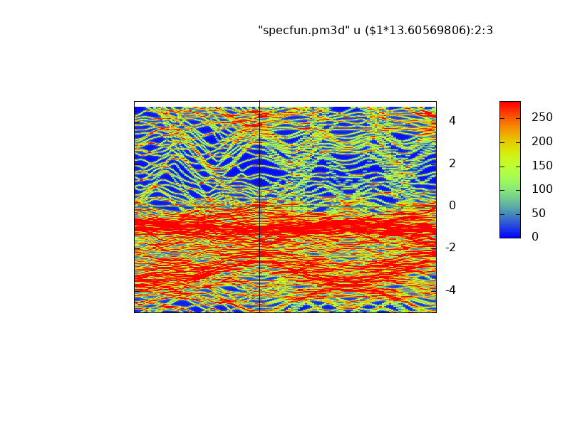
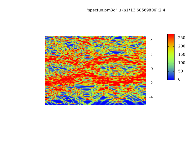
Spectral Function from lmgf
A Green’s functions does not supply quasiparticle levels, but it does contain the spectral function . The analog of the band structure can be got by drawing as a “heat map” on a grid. Since in this case there are no alloy or many-body scattering processes, the spectral function is fully coherent with unit Z factor and sharp peaks at the QP levels. They show up as bright spots on a heat map.
lmgf will make data for a heat map in lieu of the band structure, using the --band switch. By passing the Fermi level within the --band switch, lmgf will shift the spectral function to make EF coincide with 0. This is useful for comparison to the band structures drawn previously.
lmchk ctrl.asa  --syml~n=41~q=0,1,0,0,0,0,1,0,-1
mpix -n 16 lmgf ctrl.asa -vccor=f -vnit=50 -vscr=2 --pr40,21 -vgamma=t --band:fn=syml
SpectralFunction.sh  -w -5:5
open asa_UP.png
open asa_DN.png
Majority (left) and minority (right) spectral functions bands of the Nb/Fe superlattice
 .
.
 .
.
Spectral functions correspond well to the energy bands generated by lm, Note in particular the narrow Fe d bands are bunched together and show greater intensity (red). They correspond to the Fe d bands, seen as nearly flat bands in green near the Fermi level.
6. Nb/Fe/Nb Trilayer
The current system has two layers of Nb, followed by three Fe layers, followed by two more Nb layers. Since boundary conditions are periodic the geometry is
··· Nb ¦ Fe ¦ Nb ¦ Nb ¦ Nb ¦ Fe ¦ Nb ¦ Nb ¦ ···
lmpg works for a trilayer geometry:
··· Left ¦ Left ¦ Left ¦ Active ¦ Right ¦ Right ¦ Right ¦ ···
In our case Left and Right are both (3×1) reconstructed Nb. The density should correspond to that of bulk Nb, calculated in Section 1.
To make the transition, the following preparatory steps must be taken:
A PGF category must be added to the ctrl file, analogous to the GF category. This includes:
The 3rd lattice vector out of the plane must be defined for the left end lead (PGF_PLATL), and
the 3rd lattice vector out of the plane must be defined for the right end lead (PGF_PLATR).lmpg cannot yet handle inequivalent L-cutoffs. In prior sections we used LMX=1 for the E sites; this must be converted to LMX=2.
Principal layers assigned (information embedded in the site file)
For the periodic case with a larger basis, a new polarizability file constructed the self-consistent density remade
A trial restart file constructed. The one generated for the periodic case can be adapted to the trilayer case.
This step is normally taken following Section 5. To run it as a standalone test do:
~/lmf/testing/test.nbfeasa --quiet 1 2
cp ~/lmf/testing/nbfe/rsta.asa.lmgf ~/lmf/testing/nbfe/vshft.asa.gf .
test.nbfeasa will perform the steps of this section automatically, with the following:
~/lmf/testing/test.nbfeasa [--MPIK] 5
It is useful as a sanity check to check that you’ve done all the steps in the proper order.
Section 6 consists of the following steps:
a. Use blm to add PGF category to the ctrl file and also set LMX=2 (output = ctrl). b. Use lmscell to assign principal layers (site4)
c. Run lm -vscr=11 to make the static ASA response function in this basis (output = psta)
d. Run lmgf -vscr=2 to converge to self-consistency in larger basis
e. Use lmpg --rsedit to create a restart fle for a trilayer, suitable for lmpg. It imports the restart file for the active region from the periodic case created by lmgf and the restart file for padding layers from bulk Nb. (output = rsta.asa)
f. Make a starting potential from the restart file.
g. Make L- and R- end leads self-consistent
h. Make the active region self-consistent (output = rsta9.asa)
a. Remake ctrl.asa with the following:
blm --pr35 --nl=3 --pgf~platl=0,0,1~platr=0,0,1 --gf --nfile --rdsite=site7 --rdspec --usefiler --nosort --shorten=no --nk=9,4,2 --mag --asa~pfree~rmaxs=7.2 --wsite@fn=null asa --omax=.18,.26,.26
cp actrl.asa ctrl.asa
sed -i.bak -e 's/LMX=1/LMX=2 IDMOD=0,0,1/' ctrl.asa
rm ctrl.asa.bak
blm is invoked in a manner similar to the construction for the crystalline case but we do not need to worry about finding E spheres or adjusting sphere radii. We can just use what we got for the periodic case. The main addition is the --pgf switch: It tells blm to add a PGF category, specifying tags PGF_PLATL and PGF_PLATR (see here). The reconstructed Nb layers are periodic normal to the plane with lattice vector (0,0,1) (third lattice vector in site3.nbasa, Section 1.
b. Define principal layers. The principal layer technique relies on the hamiltonian being short ranged; then the matrix becomes sparse. The normal axis must be partitioned into principal layers, constructed so that the hamiltonian extends only to neighboring PL, making the hamiltonian tridiagonal in the PL.
The ASA hamiltonian is indeed short-ranged; the hamiltonian can reasonably be truncated at about 7 a.u. — second neighbors for bcc Nb and Fe (see Figures 5 and 15 of Ref. 1).
lmscell has a utility to assemble PL indices automatically given a specified range of the hamiltonian (which amount to the range of structure constants in the ASA). See here for documentation of the stack editor. The following reads structural data from site5.asa, finds the PL and writes the updated information to site3.asa:
lmscell -vpgf=1 -vfile=5 ctrl.asa --stack~setpl:withinit:rangea=1.1~wsite@fn=site4
The stack editor relies on the fact that lmscell was previously invoked with initpl, to make site5.asa.
c. Remake psta.asa in the larger basis (same steps as in Section 3).
cp rsta.asa.lmgf rsta.asa
lmstr -vfile=4 asa > out.lmstr2
touch -vfile=4 nb.asa; rm -f {nb,fe,e}*.asa save.asa mixm.asa sv.asa log.asa
lm -vfile=4 asa -vnit=-1 --pr30,20 --rs=1,0 -vscr=11 > out.psta3
d. Make a new self-consistent density in the enlarged basis
rm -f save.asa mixm.asa sv.asa log.asa vshft.asa       ← Fresh start
cp vshft.asa.gf vshft.asa                              ← Not required, but saves work since vshft for large basis similar
lmgf -vfile=4 ctrl.asa -vccor=f -vnit=50 -vscr=2 --pr40,21 -vgamma=t --rs=0,1 > out.lmgf2
lm asa --rsedit~rs~save@nopot@fn=rsta7~q > out.lm5     ← Not required, keeps restart file for self-consistent lmgf
cp rsta7.asa rsta.asa.lmgf2                            ← Restart file for self-consistent lmgf density
head -1 vshft.asa > vshft.asa.gf2                      ← Not required, preserves shift for self-consistent lmgf
e. Create a restart file for the trilayer geometry
cp rsta.asa.lmgf2 rsta.asa
cat vshft.asa.gf2 | awk '-F[= ]' '{printf " ef=%s  vconst=%s vconst(L)=%s vconst(R)=%s\n", $3,$6,$6,$6}' > vshft.asa
lmpg -vpgf=1 -vfile=4 ctrl.asa --rsedit~rs@3d~rs@ib=61@src=1:3@fn=rsta2~rs@ib=64@src=1:3@fn=rsta2~save@nopot@fn=rsta8~q > out.lmpg0
cp rsta8.asa rsta.asa.pgf0
cp rsta.asa.pgf0 rsta.asa
rm -f save.asa mixm.asa sv.asa log.asa vshft.asa
check rsta.asa.pgf0 :  max deviation (0) within tol (2e-6) of /home/ms4/lmf/b/./testing/nbfe/rsta.asa.pgf0 ? ... yes
lmpg -vpgf=1 -vfile=4 ctrl.asa -vccor=f -vnit=0 -vscr=11 --pr40,21 -vgamma=t --rs=1,0 > out.lmpg1
lmpg -vpgf=2 -vfile=4 ctrl.asa -vccor=f -vnit=0 -vscr=11 --pr40,21 -vgamma=t --rs=1,0 > out.lmpg2
The restart file editor is used in a similar manner to Section 4, apart from the new feature **rs~3d$$. For restart file editor instructions, see the Appendix.
f. Create a starting potential for both end leads and the active region. Note -vnit=0 –rs=1,0 causes lmpg to read P, Q from the restart file, make potential parameters needed to make G, and exit.
rm -f save.asa mixm.asa sv.asa log.asa vshft.asa
check rsta.asa.pgf0 :  max deviation (0) within tol (2e-6) of /home/ms4/lmf/b/./testing/nbfe/rsta.asa.pgf0 ? ... yes
lmpg -vpgf=1 -vfile=4 ctrl.asa -vccor=f -vnit=0 -vscr=11 --pr40,21 -vgamma=t --rs=1,0 > out.lmpg1
lmpg -vpgf=2 -vfile=4 ctrl.asa -vccor=f -vnit=0 -vscr=11 --pr40,21 -vgamma=t --rs=1,0 > out.lmpg2
g. Make the end leads self-consistent.
lmstr -vpgf=1 -vfile=4 asa > out.lmstr2
rm -f save.asa mixm.asa sv.asa log.asa vshft.asa
lmpg -vpgf=2 -vfile=4 ctrl.asa -vccor=f -vnit=20 -vscr=0 --pr35,21 -vgamma=t >> out.lmpg2
Note -vpgf=2, which assigns PGF_MODE to 2 (see the ctrl file). The function of that tag can be found in the documentation for lmpg, or use the on-line help:
lmpg --input | grep -A 10 PGF_MODE
h. Make the active region self-consistent. Note -vpgf=1 in this case.
rm -f save.asa mixm.asa sv.asa log.asa
/home/ms4/lmf/b/lmpg -vpgf=1 -vfile=4 ctrl.asa -vccor=f -vnit=50 -vscr=2 --zerq~all~qout --pr35,21 -vgamma=t --iactiv=no --rs=0,1 > out.lmpg
lmpg -vpgf=1 -vfile=4 ctrl.asa --rsedit~rs~save@nopot@fn=rsta9~q > out.lmpgf
The last step is not needed, but it makes compressed restart file, rsta9.asa which is sufficient to reconstruct the density. Thanks to the presence of psta.asa, convergence to self-consistency is smooth.
Appendix. ASA restart file editor instructions
This section documents the instruction set of ASA form of the restart file editor. You can operate it in interative mode or batch mode, or a mix, as you can for other editors.
To run it in interactive mode, do one of the following: lm --rsedit or lmgf --rsedit or lmpg --rsedit.
Most instructions have optional arguments. They separated by a delimiter, taken as the first character, e.g. you can use a space.
In the description below it is assumed to be @ .
Note: if you are operating the editor in batch mode, be sure to distinguish this delimiter from the batch mode delimiter.
The restart file editor can carry simultaneously two densities (1st and 2nd density); the 2nd can be combined with the first to make a new density.
Instruction set:
?
prints out a brief summary of editor’s instructions- rs[@3d | @ib=n@src=lst[@rdim[,tag,tag,…]][@fn=filnam] | rs [filnam]
Read density and associated parameters from an ASA restart file, and store in 1st density. If you do not supply a file name, rsta.ext is used for filnam.
Some elements (e.g. nuclear charge) must match what was supplied by the input file.
Options:- @3d (for lmpg): imports information from a restart file made for periodic boundary conditions into a restart file for trilayer geometry, copied into the active layer of the trilayer geometry (they should be dimensioned the same).
- ib=n@src=site-list imports ASA moments P, Q for sites in site-list contained in filnam, and copies them into the1st density, sites ib,ib+1,….
The number of sites copied is the size of site-list. site-list is an integer liste - [@rdim[,tag,tag,…]] affects parameters in the species associated with a site. By default they are left unchanged, but you can substitute the values from fnilnam. @rdim without arguments substitutes all the parameters listed below; alternatively you can use the optional tags to limit what is imported.
a : radial mesh parameter controlling spacing between points near the sphere augmentatation radius
nr : number of radial mesh points
z : atomic number
lmxa : augmentation l
class : class index
ves : electrostatic potential
rmt : sphere augmentation radius
Example: rs@fn=rsta2@rdim,a=#,z=#@ib=10,src=2:4
imports P, Q from rsta2.ext (or if it is missing, from file rsta2), sites 2,3,4, and parks them in sites 10,11,12. Also species parameters a and z are copied (changing the atomic number).
read [fn]
Read density and associated parameters from an ASA restart file, and store in 2nd density. If you do not supply a file name, rsta.ext is used for fn- set all|pnu|qnu 1|2 zers|zerq|flip
Modifies the charge or magnetic moment of a density.- The first argument specifies which objects are affected:
all applies to all quantities
pnu to the linearization parameters
qnu to the moments - The second argument refers to the first or second density
- Case third argument = zers: zeros spin part of density: n+ − n- = 0
Case third argument = zerq: zeros charge part of density: n+ + n- = 0
Case third argument = flip: exchange n+, n-
- The first argument specifies which objects are affected:
add all|pnu|qnu fac1 fac2 lst1 lst2
Store a linear combination of the two densities into the into the 1st density.
The first argument’s meaning is the same for set
The objects specified will be replaced by fac1×(1st type) + fac2×(second type)
lst1 is a site-list for the 1st density.
lst2 is a matching site list for the 2nd density, OR
lst2 is single site (same site added to all sites)exch 1|2 [flip] site1 site2
Exchanges the l=0 parts of two site densities. Optional flip flips spins during exchange.show
Show information about ASA moments P, Qsave@fn=fn | save [fn] | savea@fn=fn | savea [fn]
saves restart data in ascii restart file (name is rsta.ext unless fn is supplied.- q | a
Quits the editor.
Footnotes and references
1 Dimitar Pashov, Swagata Acharya, Walter R. L. Lambrecht, Jerome Jackson, Kirill D. Belashchenko, Athanasios Chantis, Francois Jamet, Mark van Schilfgaarde, Questaal: a package of electronic structure methods based on the linear muffin-tin orbital technique, submitted to CPC. Preprint https://arxiv.org/abs/1907.06021