The ASA layer Green's function program lmpg

This package implements a modification of the ASA Crystal Green’s function, an implemention of the Atomic Spheres Approximation adapted to layer geometry. In the layer geometry periodic boundary conditions are used in two dimensions, but not the third. Along the third axis, there is an “active” cladded by semi-infinite leads on each end, whose potential is assumed to repeat periodically in a half-plane. Thus lmpg is the layer counterpart to the crystal code lmgf.

A layer geometry makes transport calculations possible. The Landauer-Buttiker formalism has been implemented, including a capability for nonequilibrium Green’s functions.

There a tutorial showing how to translate a system set up for periodic boundary conditions into one with a geometry of the form lmpg uses.

Note: This documentation was translated from a latex document, and needs some refinement.

Table of Contents

• Definition of the layer geometry
• Green’s functions for the end regions
• Self-consistency and charge neutrality
• Electrostatics
  • Electrostatics in layer geometry
• Input for lmpg
  • Potential shifts
• Program operation
  • Use in conjunction with other programs

Definition of the layer geometry

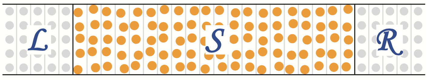
lmpg runs in much the same way as lmgf, except that lmpg has a `special direction’ which defines the layer geometry. The Green’s function G is generated in real space along this axis, and in k space along the other two. Along this axis the system is divided into a “left” semi-infinite region $\mathcal{L}$, a “right” semi-infinite region $\mathcal{R}$, and an “active” or “scattering” region $\mathcal{S}$.

.

The special axis is specified by the third primitive lattice translation vector (3^rd vector in token PLAT). For the other two axes, Bloch sums are taken in the usual way. Thus for each k in a plane defined by the first two reciprocal lattice vectors, the hamiltonian becomes one-dimensional and is thus amenable to solution in order-N time in the number of layers, as defined below.

The active region is further divided into “principal layers” 0…N−1. The left region is designated principal layer  −1; the right layer  N.

.

Layers  −1 and  N are replicated to the left and right, respectively, extending outside of the region shown. Both are replicated implicitly an infinite number of times to form the semi-infinite leads. In the “left” case a replica of each site belonging to PL −1 is translated to the left by multiples of  PLATL; similarly, a replica of each site belonging to PL  N are tranlated to the right by multiples of PLATR. PL  −1 and  N are not specified in the input file; their structures are taken from PL  0 and  N−1, translated respectively by PLATL and PLATR.

PLAT has a similar meaning in codes with periodic boundary conditions (e.g. lmgf). In that case boundary conditions are periodic in  PLAT. Thus the specification of PLAT and basis vectors inside it, whether via the ctrl file or a site file, can be identical for lmpg and lmgf.

If the left semi-infinite region covered all space (“crystal- or bulk-like”), it would be periodic with a unit cell (PLAT(1), PLAT(2), PLATL); similarly the right layer periodic with unit cell (PLAT(1), PLAT(2), PLATR). PLAT is read in the same way all programs read structural data, while PLATL, PLATR are read from the PGF category.

The central or scattering region ($\mathcal{C}$ or $\mathcal{S}$) should be constructed so that PL  −1 and  N are are already bulk-like. Thus charge densities of the PL  0 and  N−1 should rather closely resembles densities of the semi-infinite (bulk) leads. This point is discussed later.

While lmpg is similar in many respects to lmgf there is some additional complexity as a consequence of special treatment of the third dimension. To begin with, the semi-infinite layers must be specially treated in several contexts:

1. Surface analogs $\tilde G$ of $G$ for the end regions are needed to supply the boundary conditions for the embedding Green’s function. This is discussed later.

2. The left and right semi-infinite regions must be treated as periodic crystals for the special purpose of constructing the self-consistent densities and Fermi levels in those regions.

3. lmpg requires special treatment for the electrostatics joining the three regions.

Green’s functions for the end regions

By its construction the PL of each end ($\mathcal{L}-$ and $\mathcal{R}-$) region would, if repeated throughout all space, constitute a periodic solid. lmpg has a special branch for the $\mathcal{L}$ and $\mathcal{R}$ PL that enable it to generate the self-consistent left- and right- bulk G for each corresponding periodic solid.

This is needed to make the potential of each end region. Note that it is assumed to be bulk-like. The G should be the same as that generated by 3D Green’s function program lmgf, except that this G has a mixed-real and k-space representation, and separate Green’s functions and potentials are needed for each end region. Also, owing to the mixed-real and k-space representation, the methodology for constructing G is different. We will call the periodic solid of repeating $\mathcal{L}$ PL the “bulk” crystal of the $\mathcal{L}-$ region; similarly for the $\mathcal{R}$ PL. Thus, there is a well-defined “bulk” G and potential for the $\mathcal{L}$ PL, and one also for the $\mathcal{R}$ PL. A self-consistent density generated by lmpg for these regions should also be self-consistent when calculated by lmgf. In practice this becomes the case in the limit of a fine k mesh: k convergence is different in the two cases because lmpg uses only two dimensions rather than three.

You must carry out this step prior to calculations of the active region. Select this branch with PGF_MODE=2 (also see MODE=2 below).

Once the $\mathcal{L}-$ and $\mathcal{R}-$ bulk potentials are made, the surface Green’s function can be computed, which is needed to supply the proper boundary conditions to generate the GF in the embedding region.

Self-consistency and charge neutrality

Like any band method, generation of the output density requires integration to the Fermi level, which is determined by charge neutrality. Also in general, the electrostatic potential is determined up to an arbitrary constant. You can specify the Fermi level which determines the constant, or vice-versa. In the band code, we supply (or assume) the constant, and find the corresponding Fermi level. In lmgf and lmpg we indirectly fix this constant potential by specifying the Fermi level as an input. Either could serve as the independent variable for lmgf, but not lmpg because the Fermi levels of the end regions are fixed by bulk calculations.

Requirement of charge neutrality fixes the constant potential shift. Note that the GF have a complication not present in a band program, where the entire spectrum is computed: the constant shift must be determined by an iterative procedure. In the crystal GF case, it is iteratively determined by a Pade approximant (see lmgf documentation). Metals and nonmetals are distinguished in that in the latter case, there is no DOS in the gap and therefore the Fermi level (or potential shift, if the Fermi level is specified) cannot be specified precisely. As we will describe, something similar happens in the layer case, but it is a little more complicated. The Fermi level and constant potential are stored in array vshft, and permanently on disk in file _vshft._ext__{:.path} described below and in the documentation found in the source code iovshf.f.

Actually, lmpg is more general and can accommodate potential shifts at separate sites. This is useful in non-self-consistent or limited self-consistent calculations.

The layer geometry is complicated by the partitioning into three distinct regions. Self-consistency, and therefore the determination of potential, proceeds differently depending on whether one is computing the potential for the bulk $\mathcal{L}$ and $\mathcal{R}$ (PGF_MODE=2) or for the $(\ldots \mathcal{L} \vert \mathcal{C} \vert \mathcal{R} \ldots)$ layer system (PGF_MODE=1).

Computing the bulk potential for the $\mathcal{L}-$ and $\mathcal{R}-$ regions (MODE=2), is quite analogous to the crystal case, albeit for two independent regions $\mathcal{L}$ and $\mathcal{R}$. Periodic boundary conditions are assumed separately; in each case the end layer is assumed to be a periodic solid and the (periodic) Green’s function is computed for it. Thus the potential in each end layer may be shifted independently by a constant shift $V_L$ or $V_R$ . Self-consistency proceeds analogously to the crystal GF, independently for the regions $\mathcal{L}$ and $\mathcal{R}$. Constant potential shifts are determined independently for each layer in the same way as in the crystal GF code; the potential shift is computed and satisfies charge neutrality for the corresponding periodic solids; see lmgf documentation for further details. If the $\mathcal{L}$ ($\mathcal{R}$) PL is a metal, the constant potential shift is not adjustable, because the Fermi level is specified at the outset. Note, however, that the Fermi level is only sharply defined for a metal; thus it is important to distinguish metal and nonmetal cases independently in the two layers. You can set them with tokens LMET= and RMET= in the PGF category; these tokens play the role of BZ_METAL= for the crystal codes.

Charge neutrality in the layer case $(\ldots \mathcal{L} \vert \mathcal{C} \vert \mathcal{R} \ldots)$ is more complicated. It should be satisfied independently in each of the $\mathcal{L}$, $\mathcal{C}$ and $\mathcal{R}$ regions. In practice, we assume that the density in the $\mathcal{L}-$ and $\mathcal{R}-$ end regions is bulk-like and does not change once it has been calculated (MODE=2). Thus changes in the density are confined to the $\mathcal{C}-$ region. The $\mathcal{C}-$ region has to be charge-neutral because the $\mathcal{L}-$ and $\mathcal{R}-$ are already neutral, and the entire $(\ldots \mathcal{L} \vert \mathcal{C} \vert \mathcal{R} \ldots)$ system must be neutral. The program proceeds by finding a shift that satisfies charge-neutrality in the $\mathcal{C}-$ region and doesn’t worry about the rest. This is reasonable since we assume at the outset that the $\mathcal{C}-$ region has enough PL near $\mathcal{L}-$ and $\mathcal{R}-$ to allow the density to be bulk-like, no charge should spill into the $\mathcal{L}-$ and $\mathcal{R}-$ regions by construction. Thus, when computing the Green’s function of the $(\ldots \mathcal{L} \vert \mathcal{C} \vert \mathcal{R} \ldots)$ system in practice, the layer code selects the shift $V_C$ so as to eliminate the deviation from charge neutrality in the $\mathcal{C}-$ region, following the method of the crystal code lmgf. Only sites in the $\mathcal{C}-$ region are shifted by $V_C$; the potentials and charges in the $\mathcal{L}-$ and $\mathcal{R}-$ regions are left untouched. Once $V_C$ is found and the corresponding Green’s function is generated, lmpg returns to the sphere program where it computes the potential functions for the updated sphere charges and moments, computes the electrostatic potential (see below) for the $(\ldots \mathcal{L} \vert \mathcal{C} \vert \mathcal{R} \ldots)$ system, and begins another pass in the self-consistency cycle.

Because of deviations from self-consistency, and also because of finite-size effects discussed above, there can be some deviation from charge neutrality in the end regions. lmpg will generate the GF in each end PL, so that the deviation from neutrality may be computed. (You must have the ‘bigemb’ option set for lmpg to generate this information.) The sphere charges are shown in the table headed by the lines:

PGFASA: integrated quantities from G
    PL      D(Ef)      N(Ef)       E_band      2nd mom      Q-Z

and deviations of the end regions from charge neutrality are summarized at the end of this table in lines similar to the following:

Deviations from charge neutrality:
  Left end layer       0.003965
  Right end layer      0.003965

However, lmpg does not use this information; instead it keeps the densities as computed for the bulk $\mathcal{L}-$ and $\mathcal{R}-$ crystals. If these charges are not small, your active region should be enlarged.

Electrostatics

At self-consistency there is a unique potential defined by the electrostatic potential from the charges at each site and a global constant potential shift $V_C$ that shifts the entire system. This shift makes each region charge neutral and possesses within the $\mathcal{C}-$ region a dipole that will exactly align the Fermi levels in the $\mathcal{L}-$ and $\mathcal{R}-$ regions, as we now describe.

For now let’s restrict ourselves to the case when both $\mathcal{L}-$ and $\mathcal{R}-$ regions are metals. We can compute electrostatic potentials in the $\mathcal{L}-$ and $\mathcal{R}-$ regions by two different constructions:

Electrostatic potentials in $\mathcal{L}-$ and $\mathcal{R}-$ may be computed as in MODE=2, that is by assuming $\mathcal{L}-$ and $\mathcal{R}-$ are bulk solids with periodic boundary conditions in the respective $\mathcal{L}-$ and $\mathcal{R}-$ regions. In each case the potential is completely fixed by charge neutrality. Electrostatic potentials in $\mathcal{L}-$ and $\mathcal{R}-$ may also be computed from solution of the potential of the entire $(\ldots \mathcal{L} \vert \mathcal{C} \vert \mathcal{R} \ldots)$ system. This potential is adjustable up to some constant shift. In practice these two constructions produce different potential in the $\mathcal{L}-$ and $\mathcal{R}-$ regions. (Indeed, one might choose the constant shift that 'best reconciles' the mismatch in these two constructions. Versions of lmpg earlier than 6.14 did something like this. The present version chooses the constant shift so as to satisfy charge neutrality in the $\mathcal{C}-$ region, as was discussed in the previous section.)

These potentials might be mismatched for two distinct reasons. One error can arise because the density is not self-consistent. More exactly the density doesn’t possess the requisite dipole, so that a global constant shift that 'best reconciles' the potential mismatch as constructed by the two methods above is different from the one that ‘‘best reconciles’’ the mismatch on the right. Finite-size effect (a $\mathcal{C}-$ region with insufficient PL near the end regions) is another source of error.

Recall that lmpg freezes the potentials in the $\mathcal{L}-$ and $\mathcal{R}-$ regions. Thus, only the central region is affected by the shift $V_C$ because the end PL shouldn’t be shifted at all. lmpg does print out the electrostatic potentials computed by the two different constructions, and summarizes the deviations in a table similar to the following:

Deviations in end potentials:
region met  <ves>Bulk   <ves>layer     Diff      RMS diff
 L      T    0.055210    0.058192    0.002982    0.011265
 R      T    0.055210    0.058192    0.002982    0.011265

RMS pot difference in L PL = 0.000127  in R PL = 0.000127  total = 0.000127
vconst that minimizes potential mismatch to end layers =  0.058835
vconst is now (estimate to satisfy charge neutrality)  =  0.061817
difference                                             = -0.002982

The top table compares the average electrostatic potential in an end region computed from the bulk geometry, and computed in the (… $\mathcal{L}$ | $\mathcal{C}$ | $\mathcal{R}$ …) geometry. The later numbers compare the potential that ‘‘best reconciles’’ the the methods of computation to the potential shift the program will actually use. Note that the potential shift you actually should use is the one that meets charge-neutrality in the $\mathcal{C}-$ region; indeed lmpg will find this shift on its own if you invoke it in self-consistent mode (sec XX).

When getting started, this table gives you a pretty reasonable guess at the proper choice of the constant shift $V_C$. That is, you might set $V_C$ as the one that minimizes potential mismatch to end layers. You can adjust if you start out with the choice $V_C$ by invoking lmpg in an interactive mode, or by setting file vshft appropriately. If you do so, you will alleviate some of the burden on lmpg in determining this shift.

If the potential in either the $\mathcal{L}-$ or the $\mathcal{R}-$ differs significantly (see case $\mathcal{L}-$ and $\mathcal{R}-$ are both metals, below), or if there is significant deviation from charge neutrality in the end PL, the user should enlarge the embedding region, as the end PL are not sufficiently bulk-like. This difference should vanish at self-consistency if you construct the embedding region with PL near the end regions similar to those of the last region. Typically having 2 PL (say $0\ldots 1$, and $N-2\ldots N-1$ does a pretty good job keeping the discrepancies between the bulk- and layer potentials small.

Now we must distinguish between metal and nonmetal cases. If either end layer is a nonmetal, its potential can shift by a constant without affecting charge neutrality. Therefore, if either $\mathcal{L}-$ or $\mathcal{R}-$ regions is a nonmetal, there can be a constant shift in that region (change in band offset). Consider the following cases:

• $\mathcal{L}-$ and $\mathcal{R}-$ are both metals. No potential shifts are allowed in the end layers. In the self-consistency cycle (MODE=1) the program checks for deviations from charge neutrality and adjusts the potential in the $\mathcal{C}-$ region until neutrality is achieved. However, the density resulting from this Green’s function will generate charges and electrostatic potentials $V^i_m$ at sites $i$ in the $\mathcal{L}-$ and $\mathcal{R}-$ layers. As mentioned above, potentials computed from the (… $\mathcal{L}$ | $\mathcal{C}$ | $\mathcal{R}$ …) system will reveal some differences relative to the electrostatic potentials $V^i_b$ when computed using just the $\mathcal{L}-$ or $\mathcal{R}-$ charges and a geometry for infinitely repeating $\mathcal{L}-$ and $\mathcal{R}-$ layers. The potentials calculated these two ways is printed out, as described above.

• Only one of $\mathcal{L}-$ or $\mathcal{R}-$ is a metal (LMET=f and RMET=t or vise-versa). Now the nonmetallic end region can shift its potential by a constant to best align to the potential computed from the (… $\mathcal{L}$ | $\mathcal{C}$ | $\mathcal{R}$ …) system. We choose the constant in the nonmetallic PL that best aligns $V^i_b$ and $V^i_c$; that is, that minimizes the RMS difference $V^i_b$ and $V^i_c$.

• Neither the $\mathcal{L}-$ or $\mathcal{R}-$ is a metal (LMET=f and RMET=f). If the $\mathcal{C}$ region is a metal (specified by BZ METAL=) the global potential shift should conform to the shift in the $\mathcal{C}$ region. Both endpoints must be allowed to float (there are two distinct band offsets). If no region is a metal, i.e. if there is no DOS at the Fermi level, the system should already be charge neutral and no shifts should be required.

Electrostatics in layer geometry

The correct procedure to construct electrostatics in a layer geometry is to carry out 2D Ewald summations for each PL, and add up the contributions from all PL. This is described in the paper by Parry Surf. Sci. 49, 433. Since we haven’t yet made 2D Ewald sums for this program, we use a trick.

We compute the electrostatics via a 3D Ewald summation of the following supercell:

.

It assumes periodic boundary conditions of period in the layer direction PLAT(3) + 2×(PLATL + PLATR). There is an artificial periodicity in the boundary condition on this axis that has to be removed to make it similar to the 2D Ewald summation. There is also a small error in that the electrostatics from layers 3×PLATL and 3×PLATR, …, are omitted.

Input for lmpg

This section describes input specific to lmpg. Much of the Green’s function specific part of lmpg’s input is the same as input to the crystal Green’s function] lmgf, e.g. the  BZ_EMESH  tag.

Each site must be assigned a 'principal layer index’ to tell lmpg which principal layer a site belongs to. Each member of category SITE, should have a token PL:

Sites with the same PL index are grouped together into a single principal layer.

Note: the principal layers should be large enough such that the range of the hamiltonian connects only adjacent PL. The range of the hamiltonian is fixed by the range of the structure; you can set it manually with STR_RMAX.

There is a lmpg-specific category, which includes the following:

PGF    MODE=#
       PLATL=#1 #2 #3
       PLATR=#1 #2 #3
       GFOPTS=options
       SPARSE=#

MODE, PLATL, and PLATR are required inputs.

MODE tells lmpg what to do:

• #=0: do nothing after the atomic part
• #=1: calculate the diagonal part of G, layer-by-layer. This is the appropriate mode for self-consistent calculations.
• #=2: left- and right layer “bulk” Green’s functions, equivalent to crystal Green’s functions for the left and right leads. This mode is designed to generate a self-consistent densities for left- and right- leads as though they were crystalline, with periodicity given by PLATL or PLATR. lmpg must be run in this mode first.
• #=3 find k(E) for left bulk, meaning the left end layer as if it were repeated an infinite number of times in both directions. This uses a special trick (see PRB 39, 923 (1989)) to find the wave numbers of the left bulk G corresponding to a given energy. This mode is illustrated for a free-electron test case in the the step potential tutorial.
• #=4 find k(E) for right bulk.
• #=5 Calculate conductance from the Landauer-Buttiker theory. /tutorial/lmpg/steplmpg/#transmission This mode is illustrated in a tutorial for a simple flat potential with a barrier of finite width [the step potential tutorial].
• #=7 Calculate reflectance from the Landauer-Buttiker theory
• #=8 Calculate spin torques

PLATL and PLATR specify $\mathcal{L}$ and $\mathcal{R}$ specific parts of the lattice vectors for the (… $\mathcal{L}$ | $\mathcal{C}$ | $\mathcal{R}$ …) geometry

SPARSE=T tells lmpg to compute G using LU decomposition. The default is to compute G layer-by-layer via a Dyson equation (SPARSE=F)

Potential shifts

File _vshft._ext__{:.path} holds information about potential shifts as described in previous sections. The global shifts are contained in the first line and keep information about Fermi level, the global constant shift, and the shifts at the $\mathcal{L}$ and $\mathcal{R}$ end regions needed to match the Fermi level. The syntax for the first line is

ef=# vconst=# vconst(L)=# vconst(R)=#

You can optionally add site-dependent potential shifts. After the first line, add a line site shifts followed by as many lines as desired, one line per site shift, e.g.:

ef=.03 vconst=-.01 vconst(L)=.02 vconst(R)=.03
site shifts
 3    .1
 4    .2

Program operation

lmpg starts by creating the left surface, and then proceeds ‘left-to-right’ layer-by-layer to generate the surface GF for PL 0,1,2,3,… until the rightmost layer is reached. At that point the right surface GF is generated, and the crystal GF is generated by embedding between the left- and right- surface GF.

Then using Dyson’s equation, lmpg proceeds layer-by-layer ‘right-to-left’ to generate the crystal GF from the surface GF on the left and the crystal GF on the right. This is done for each energy and k-point in the two-dimensional Brillouin zone.

Use in conjunction with other programs

You can use plane-analysis tool lmplan to analyze charge distributions by plane, and also use it to create a site file to facilitate making of lattices with periodic boundary conditions so that you can run lm and lmgf for comparison.

Note: This documentation is outdated and needs revision.

At present lmpg cannot make the static response function, as lmgf can; this can vastly improve effiency for self-consistency. However, if you make the response function using lmgf, you can use it with the lmpg program. Here is an example taken from the directory of pgf/tests/copt.

Invoke this command

lmplan copt -vpgf=1 -cstrx=file -vlmf=f -vnk1=6 --pr31 -vnit=10 -vgamma=f -vsparse=0

At the prompt, type

wsite -pad abc

lmplan creates a site file named ‘abc.copt’ suitable for use with programs lm and lmpg. It uses the padding layers as buffer layers. Conveniently, it satisfies periodic boundary conditions. To verify this, try

cp abc.copt site.copt
lmchk copt -vpgf=0 -cstrx=file -vlmf=f -vnk1=6 -pr31 -vnit=10 -vgamma=f -vsparse=0

Now you can make a suitable ASA static response function suitable for the layer code with

lmgf copt -vpgf=0 -cstrx=file -vlmf=f -vnk1=6 -pr31 -vnit=10 -vgamma=f -vsparse=0 -iactiv -time=5 -vscr=1

The q=0 response function is written to file _psta._ext__{:.path}. (This file has already been created and sits in pgf/test/copt.) Once the psta is created, it can greatly facilitate convergence to self-consistency. Try running, for example, the test script

pgf/test/test.pgf -usepsta copt 5

will use the psta file to assist convergence when you use the switch -usepsta. Look in particular at the RMS DQ, viz:

grep RMS out.lmpg.self-consistent

PQMIX:  read 0 iter from file mixm.  RMS DQ=1.84e-3
PQMIX:  read 1 iter from file mixm.  RMS DQ=1.59e-4  last it=1.84e-3
PQMIX:  read 2 iter from file mixm.  RMS DQ=3.30e-4  last it=1.59e-4
PQMIX:  read 3 iter from file mixm.  RMS DQ=4.66e-5  last it=3.30e-4

If you invoke it in the usual way, viz without -usepsta:

PQMIX:  read 0 iter from file mixm.  RMS DQ=1.44e-3
PQMIX:  read 1 iter from file mixm.  RMS DQ=6.41e-3  last it=1.44e-3
PQMIX:  read 2 iter from file mixm.  RMS DQ=2.22e-1  last it=6.41e-3
PQMIX:  read 3 iter from file mixm.  RMS DQ=3.05e-2  last it=2.22e-1
PQMIX:  read 4 iter from file mixm.  RMS DQ=3.01e-2  last it=3.05e-2
PQMIX:  read 5 iter from file mixm.  RMS DQ=2.66e-2  last it=3.01e-2
PQMIX:  read 6 iter from file mixm.  RMS DQ=4.15e-2  last it=2.66e-2
PQMIX:  read 7 iter from file mixm.  RMS DQ=4.92e-2  last it=4.15e-2
PQMIX:  read 8 iter from file mixm.  RMS DQ=4.40e-2  last it=4.92e-2
PQMIX:  read 8 iter from file mixm.  RMS DQ=2.24e-2  last it=4.40e-2