Including Ladder Diagrams in W
This tutorial will go through how to run a QSGW calculation whilst including ladder diagrams (vertex contributions) in the screened Coulomb interaction W. By default, Questaal will perform a QSGW calculation with the polarization calculated at the level of the random phase approximation (RPA). This is calculated in the program hx0fp0 (hx0fp0_sc). To include ladders in W, the RPA W is first calculated in hx0fp0 and this is then used in the Bethe-Salpeter equation (BSE) for the full polarization matrix (See this page for a background to the theory). The BSE for the improved W is calculated by the program bethesalpeter, which is included in the QSGW calculation with the switch UseBSEW set to 1 in GWinput (see below). The new W is then used instead of the RPA W in hsfp0 (hsfp0_sc) to calculate the screened part of the self-energy.
Command Summary
bsub -Is -n 24 -q scarf-rhel7 -R "span[hosts=1]" /bin/bash
module use /home/cseg/scarf590/opt/modules/o
module load workshop
mkdir NiO
cd NiO
cp /home/cseg/scarf590/dev/201805m/lm/gwd/test/nio.code/{ctrl.nio,rst.nio,sigm.in,switches-for-lm,basp.nio,site.nio,EPS0001.dat} ./
mv sigm.in sigm
ln -s sigm sigm.nio
lmf -vnit=1 --iactiv=no `cat switches-for-lm` ctrl.nio > out.lmf_QSGW
lmchk ctrl.nio  `cat switches-for-lm` --syml~mq~lbl=XGLUT~q=0,1/2,1/2,0,0,0,0,1/2,0,11/32,26/32,11/32,1/2,1/2,1/2
lmf -vnit=1 --rs=1,0 `cat switches-for-lm` --band:fn=syml ctrl.nio
cp bnds.nio bnds.qsgw
lmf -vnit=1 --rs=1,0 -vloptic=1 -vmetal=3 `cat switches-for-lm` ctrl.nio # produces RPA absorption (see below)
echo -1 | lmfgwd `cat switches-for-lm` ctrl.nio
nano GWinput # Change UseBSEW, NumCondStates and add NumValStates (see below)
lmgwsc --iter=1 --maxit=1 --code2 --openmp=16 --sym --getsigp --insul=22 nio > out.lmgwsc_bse
lmf -vnit=12 --iactiv=no `cat switches-for-lm` ctrl.nio > out.lmf_QSGWBSE
lmf -vnit=1 --rs=1,0 `cat switches-for-lm` --band:fn=syml ctrl.nio
cp bnds.nio bnds.bse
echo -9,16 / | plbnds -ef=0 -scl=13.6058 -fplot -lbl=X,G,L,U,T bnds.nio
fplot -f plot.plbnds
Preliminaries
lmf, lmfgwd, lmgwsc are all assumed to be in your path. The source code for all Questaal executables can be found here.
You should ensure that the executable bethesalpeter is also in your path.
Tutorial
Start by connecting to the compute nodes, load the necessary modules and make a directory NiO
$ bsub -Is -n 24 -q scarf-rhel7 -R "span[hosts=1]" /bin/bash
$ module use /home/cseg/scarf590/opt/modules/o
$ module load workshop
$ mkdir NiO && cd NiO
We start this calculation from a converged QSGW calculation; some of the steps in this tutorial wont be necessary if you performed the calculation from scratch and these will be highlighted. The screening W in the converged calculation was calculated in the RPA, hence the large band gap overestimation (see below). The ctrl.nio, site.nio, basp.nio and switches-for-lm files are all located in ~path-to-questaal/lm/gwd/test/nio.code2/. switches-for-lm contains command line arguments that can be changed such as the number of k-points, the maximum number of iterations, etc. The QSGW self-energy that is read by lmf is also contained in this directory and called sigm.in. Finally the file rst.nio that is needed for this calculation is contained in this directory. These files would all be produced if one had started this calculation from scratch (See this page on how to run a basic QSGW calculation for Si). The sigm file that is read by lmf is called sigm.nio and, again, this file would have been created by the script lmgwsc.
$ cp /home/cseg/scarf590/dev/201805m/lm/gwd/test/nio.code2/{ctrl.nio,rst.nio,site.nio,switches-for-lm,basp.nio,sigm.in,EPS0001.dat} ./
The path to Questaal executables can be found by typing the command which lmf. The EPS0001.dat file contains the macroscopic dielectric function (columns 5 and 6 for the real and imaginary parts) as a function of energy in Rydbergs (column 4). Note that it may be necessary for plotting purposes to run the command
$ sed -i -e 's/D/E/g' EPS0001.dat
so that exponents in this file are written with an E instead of D. We copy this file to compare with other methods for calculating the macroscopic dielectric function below.
The file sigm.in created in lmgwsc would actually be called sigm.nio and lmgwsc would have created a link to sigm. To do this here we type
$ mv sigm.in sigm
$ ln -s sigm sigm.nio
Now run lmf to produce the H0 and neccessary files needed for GW
$ lmf --iactiv=no -vnit=12 `cat switches-for-lm` ctrl.nio > out.lmf_QSGW
The –iactiv=no turns off the interactive mode and -vnit=12 means the calculation will perform a maximum of 12 SCF iterations. Note that if these switches are placed before the catswitches-for-lm command then these values will take precedence over the values in switches-for-lm, however, if the are placed after then the values in the file will be used.
If we grep for the bandgap (grep gap *), we should find that lmf produces a bandgap of 4.86 eV, an overestimate of 0.5~0.6eV with respect to experiment. A QSGW band structure can be produced following the usual steps, which are discussed below.
We will now create the file needed for plotting the band structure. To produce the syml.nio file containing the high-symmetry points and paths around the Brillouin zone, run the command
$ lmchk ctrl.nio `cat switches-for-lm` --syml~mq~lbl=XGLUT~q=0,1/2,1/2,0,0,0,0,1/2,0,11/32,26/32,11/32,1/2,1/2,1/2
then produce the band structure in the usual way
$ lmf -vnit=1 --rs=1,0 `cat switches-for-lm` --band:fn=syml ctrl.nio
$ cp bnds.nio bnds.qsgw
We can also produce an RPA optical absorption spectrum here using lmf. The necessary categories should be in the ctrl.nio file. To do this run
$ lmf --iactiv=no -vnit=1 --rs=1,0 -vmetal=3 -vloptic=1 `cat switches-for-lm` ctrl.nio
The extra switches are discussed below. The file opt.nio is produced which contains 7 columns: energy (Ry), followed by the diagonal elements of the dielectric tensor (x,y,z components) for both spin channels. This can be compared with EPS0001.dat
Next we produce the files necessary for the GW calculation
$ echo -1 | lmfgwd `cat switches-for-lm` ctrl.nio
If we run lmgwsc as is then lmgwsc will perform a GW calculation with the W calculated within the RPA. To include ladder diagrams in W we need to edit GWinput and change/add the token UseBSEW 1
$ nano GWinput
UseBSEW   1
NumCondStates 11
NumValStates 16
The NumValStates and NumCondStates categories are the number of valence and conduction states considered in the BSE. Since the BSE is rather expensive (in compuational time and memory) all transitions between states cannot be considered at this level. States within a particular energy window about the Fermi level are considered in the BSE; the rest are treated at the level of the RPA. For this tutorial, 16 Valence and 11 conduction states are enough to demonstrate the method. There are other parameters that can be changed that affect the BSE program and some of these (along with their defaults and a description) are listed below:
ImagEner1 0.02 ! Broadening in Rydberg (~0.25eV)
ImagEner2 0.02 ! Broadening at Max Omega (see file freq_r). Broadening increases linearly from ImagEner1 at omega=0
NumValStates2 Nv2 ! Number of valence states in BSE for spin channel 2
NumCondStates2 Nc2 ! As above, but for the conduction states
Gauss_BSE off ! if on, use Gaussian broadening for the imaginary part of epsilon.
Gauss_cutoff 0.0 ! Gaussians used up to this cut-off, ensures the peaks aren't broadened too much near omega=0
Next we perform one iteration of QSGW with ladder diagrams now included in the screening.
$ lmgwsc --iter=1 --maxit=1 --code2 --openmp=16 --sym --getsigp --insul=22 nio > out.lmgwsc_bse
The switches are the usual lmgwsc ones. N is the number of processors you wish to use in the calculation. In the file out.lmgwsc_bse we see that the output from the bethesalpeter code is directed to the file lbse. The RMS change in Sigma (see the bottom of out.lmgwsc_bse) is about 5.3E-3. This is a way of comparing H0 and H, i.e., comparing the QSGW Sigma without ladders in W and the case with ladders. Another iteration of lmgwsc reduces the calculated bandgap from 4.61 eV (see below) to 4.45 eV, and this is done by changing the switch –maxit=2 in the command above.
Using the new sigm file created we can now run lmf and see how the band gap has changed.
$ lmf -vnit=12 --iactiv=no `cat switches-for-lm` ctrl.nio > out.lmf_QSGW_BSE
We find that the gap has reduced to 4.61 eV (from 4.86 eV). We can now produce a band structure from this converged density.
Band Structure
The band structure can be produced in the usual way. In this example we follow the method on this page to produce a plot comparing band structures at different levels of theory (in this case QSGW(RPA) and BSE on top of QSGW). Note that we use ghostscript to view the postscript:
$ lmf -vnit=1 --rs=1,0 `cat switches-for-lm` --band:fn=syml ctrl.nio
$ cp bnds.nio bnds.bse
$ echo -9,16 /  | plbnds -wscl=1,.8 -fplot -ef=0 -scl=13.6 --nocol -lbl=X,G,L,U,T -spin2 -dat=bse bnds.bse
$ echo -9,16 /  | plbnds -wscl=1,.8 -fplot -ef=0 -scl=13.6 --nocol -dat=qsgw -spin2 bnds.qsgw
$ echo "% char0 colr=3,bold=5,clip=1,col=1,.2,.3" >>plot.2bands
$ echo "% char0 colb=2,bold=4,clip=1,col=.2,.3,1" >>plot.2bands
$ awk '{if ($1 == "-colsy") {sub("-qr","-lt {colg} -qr");sub("dat","green");sub("green","bse");sub("colg","colr");print;sub("qsgw","bse");sub("colr","colb");print} else {print}}' plot.plbnds >> plot.2bands
$ fplot -f plot.2bands
$ gs fplot.ps
The plot below has the vertex corrected QSGW in red (after one iteration of QSGW with BSE) and bare QSGW in blue (note these may be swapped?). 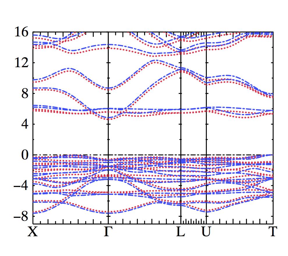
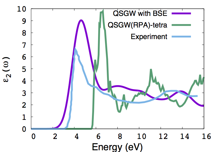
Optical absorption spectrum
See this page for a description of how to calculate an optical absorption spectrum for LiF. A list of commands are presented below for producing one for NiO. Edit the OPTICS catergory in ctrl.nio to calculate the transition dipole matrix elements (TDMEs) needed for the macroscopic dielectric function
$ nano ctrl.nio
OPTICS
  MODE=1
  LTET=0
  WINDOW=0 4
  NPTS=1001
  FILBND=1 22
  EMPBND=23 100
  MEFAC=1
MEFAC=1 will include a contribution to the TDMEs from the self-energy (see Phys. Rev. Mat. 2, 034603). Note that lmf cannot run with MEFAC=1 and -vmetal=5 (in switches-for-lm) together. Therefore we change -vmetal to 3.
The set of commands to calculate the TDMEs are
$ echo 6 | lmfgwd `cat switches-for-lm` ctrl.nio # Ensures q-points and phases are the same between lmf and lmgw
$ lmf -vmetal=3 --opt:woptmc:permqp --revec:gw -vnit=1 --rs=1,0 -vloptic=1 `cat switches-for-lm` ctrl.nio
$ cp optdatac.nio optdatabse # optdatabse is the file read by bethesalpeter
Edit the GWinput for the calculation of the absorption:
$ nano GWinput
NumCondStates 11 !
Qvec_bse 0 0 1  ! q-vector direction
NumValStates 16
MaxOmega_BSE 2.0
MinOmega_BSE 0.0
numOmega_BSE 2001
Gauss_BSE on
ImagEner1 0.05 ! Large broadening to match experiment!
Now run
$ echo -1 | /home/cseg/scarf590/dev/201805m/lm/b-o/code2/bethesalpeter > out.rpa # Produces an RPA absorption spectrum, which can be compared with that in EPS0001.dat
$ cp eps_BSE.out eps_RPA.out
$ export MKL_NUM_THREADS=8
$ echo 0 | /home/cseg/scarf590/dev/201805m/lm/b-o/code2/bethesalpeter > out.bse
The absorption spectrum is written to the file eps_BSE.out, with 3 columns: energy (eV) followed by the real and imaginary part of the macroscopic dielectric function. Note the blue shift w.r.t. experiment, which can be reduced if we further iterate the QSGW including ladder diagrams, and if we could include the electron-phonon contribution to W. We plot eps_BSE.out against the experiment and the RPA QSGW spectrum from the file EPS00001.dat