lmgf-cpa tutorial

This tutorial explains how to use the Coherent Potential Approximation (CPA) in the ASA Green’s function code lmgf. The CPA models disorder by treating a single site as a collection of atoms.

This code implements two forms of CPA: atomic disorder and spin disorder.

If you haven’t yet done so, you are advised to go through the Introductory lmgf tutorial before trying this one.

Copy the input file ctrl.perma

Make a self-consistent potential

lmstr perma vnit=1 -vxcu=0.2 -vcfe=0.2 --pr35,25
lmgf perma -vnit=0 -vxcu=0.2 -vcfe=0.2 --pr35,25
mpix -n 16 lmgf perma -vnit=100 -vxcu=0.2 -vcfe=0.2 -vgamma=4 --pr35,25 > out
mpix -n 16 lmgf  perma -vnit=1 -vxcu=0.2 -vcfe=0.2 -vgamma=4 --pr35,25 --rs=0,1

Make the Ω potential on the real axis

mpix -n 16 lmgf perma -vsc=0 -vnit=1 -vgamma=4 -vxcu=0.2 -vcfe=0.2

Make the spectral function on the real axis, on given symmetry lines. You will need syml.perma

lmgf  perma -vsc=-1 --band:fn=syml -vnit=1 -vgamma=4 -vxcu=0.2 -vcfe=0.2

Preliminaries
Building the ctrl file
Spectral function calculations with lmgf
- Plotting the spectral function
Footnotes and references

Preliminaries

For this tutorial the Questaal binaries lmstr, and lmgf executables are required and are assumed to be in your PATH; the source code for all Questaal executables can be found here.

This tutorial also assumes you are working with an MPI version of lmgf. Here we use mpix as a proxy for your MPI program (typically mpirun). You can use as many processors as convenient. You can also run in serial mode by omitting the mpix -n 16 where it appears.

This tutorial was adapted from the paper in Reference 1.

Building the ctrl file

The CPA documentation should explain all the steps we’re going to take; we advise you to read it before starting the tutorial.

First of all we need a control file adapted for CPA case. Copy the contents of the box below into file ctrl.perma.

# Lattice constant 3.57A (taken from RT data in Stremme's PhysLettA46) reduced by 0.2%
# Choose sc=1 for self-consistency, sc=0 for omega=sc on real axis, sc=-1 for spectral function
% const sc=1
% const a=6.73 nk=16 nl=3 cfe=.20 cni=1-cfe xcu=0 # xcu=0 => 2 components only
HEADER  Alloys of Fe and Ni with other elements
VERS    LMASA-7.0 LM:7 ASA:7 LMGF:7
IO      SHOW=F HELP=F VERBOS=31,20 WKP=F IACTIV=F
% const gamma=2
OPTIONS ASA[CCOR=F GAMMA={gamma} TWOC=F]
HAM 	NSPIN=2 REL=T BXCSCAL=1
STR
BZ      TETRA=T NKABC={nk} METAL=1 BZJOB=0 INVIT=F
%ifdef sc==1
        EMESH=51 10 -.85 0 .4 0   # For self-consistency
%endif
        EMESH=501 2 -.5 .2  .001 0   #for dos
STRUC   NBAS=1 NSPEC=3 NL={nl}
        ALAT={a} PLAT=  0 .5 .5  .5 0 .5  .5 .5 0
SPEC
%ifdef xcu==0
        ATOM=Fe R/W=1 Z=26 CPA=1 2 C={cfe} {cni} MMOM=0,0,2
%else
        ATOM=Fe R/W=1 Z=26 CPA=1 2 3 C={cfe}*{1-xcu} {cni}*{1-xcu} {xcu} MMOM=0,0,2
%endif
        ATOM=Ni R/W=1 Z=28 MMOM=0,0,1
        ATOM=Cu R/W=1 Z=29
SITE    ATOM=Fe POS=0 0 0
%const  nit=1
ITER    NIT={nit}  MIX=B5,b=0.1 CONV=1e-6 CONVC=1e-6
START   CNTROL=F BEGMOM=T
%const  gfmod=1
GF      MODE={gfmod} DLM={sc==1?12:32}
%ifdef sc==1
        GFOPTS=p3;padtol=.001;omgmix=0.4;padtol=1d-3;omgtol=1d-3;lotf;nitmax=30
% elseifd sc==0
        GFOPTS=p3;omgmix=0.4;padtol=0.001;omgtol=1d-6;lotf;nitmax=50
% else
        GFOPTS=p3;specfr;omgmix=0.4;padtol=0.001;omgtol=1d-6;lotf;nitmax=50
% endif
START   BEGMOM=T

Check the CPA documentation here. It explains carefully the additions to a control file required to turn on chemical and/or magnetic CPA. Additional species must be defined for chemical CPA, and their concentrations. It’s done in the SPEC category in the following way:

SPEC ATOM CPA= and C= together turn on chemical CPA for a particular species.

Look into control file. There we have

        ATOM=Fe R/W=1 Z=26 CPA=1 2 3 C={cfe}*{1-xcu} {cni}*{1-xcu} {xcu} MMOM=0,0,2
        ATOM=Ni R/W=1 Z=28 MMOM=0,0,1
        ATOM=Cu R/W=1 Z=29

It tells the code that our alloy consists of Fe, Ni and Cu, provides their atomic numbers. The first of the three lines also gives the concentrations for each of the elements: 1, which is Fe, for instance has concentration {cfe}*{1-xcu}. It is determined from the chemical formula $(\mathrm{Ni}_{1-cfe}\mathrm{Fe}_{cfe})_{1-xcu}\mathrm{Cu}_{xcu}$ and means we can vary the Cu and Fe concentrations from the control line. By default we have no Cu and 20% of Fe (see ctrl.perma):

% const a=6.73 nk=16 nl=3 cfe=.20 cni=1-cfe xcu=0

You can also see that we force some initial moment on Fe and Ni (see discussion of the --mag switch in the Introductory tutorial. Token GF_DLM The following token turns on the CPA and/or disordered local moments (DLM), and controls what is being calculated.

DLM=12: normal CPA calculation; both charges and Ω's are iterated
DLM=32: no charge self-consistency; only CPA it iterated until Ω reaches prescribed tolerance for each z-point.

If you look into the ctrl file you’ll see that we have both there: 12 and 32 depending on the kind of self-consistency we need since we’ll need to run it with each DLM = 12 and 32 one after another.

Same way as in for example the Introductory lmgf tutorial (please try that tutorial first if you haven’t yet done so) you’ll need to create the structure file by doing (we’re going to run a set up for $(\mathrm{Ni}_{80}\mathrm{Fe}_{20})_{80}\mathrm{Cu}_{20}$ ) and starting potential:

lmstr perma vnit=1 -vxcu=0.2 -vcfe=0.2 --pr35,25
lmgf perma -vnit=0 -vxcu=0.2 -vcfe=0.2 --pr35,25

Make the system self-consistent and do one final iteration to save the sphere moments in file rsta.perma

mpix -n 16 lmgf perma -vnit=100 -vxcu=0.2 -vcfe=0.2 -vgamma=4 --pr35,25 > out
mpix -n 16 lmgf  perma -vnit=1 -vxcu=0.2 -vcfe=0.2 -vgamma=4 --pr35,25 --rs=0,1

Note that the output ends with ‘Jolly Good Show’ … if not you may need more iterations.

Self-consistency proceeds in a triply nested loop.

Inner loop: CPA consistency. The CPA potential (configurational average of potential functions from the real atoms that occupy a particular site) must be iterated. This “coherent interactor” $\Omega$ is written to file omega1.perma, and it is frequency-dependent, but not k dependent.
Charge neutrality: the Fermi level $E_F$ must be determined for a given potential. Since the frequency mesh must be updated when $E_F$ changes, the coherent interactor must be recalculated for the new mesh.
Charge self-consistency.

Because of the complex nature of self-consistency, the charge mixing must be set fairly conservatively (ITER_MIX beta=0.1). Convergence to self-consistency is rather slower than it is in a crystalline case.

Spectral function calculations with lmgf

The ability to generate and plot spectral functions were implemented in lmgf v7.10 by Bhalchandra Pujari and Kirill Belashchenko. The details of the theory in the CPA case can be found in Ref. 2.

Please read carefully the CPA-documentation; it expains why you’ll need to run the following commands. The spectral function can be calculated for any potential, but it is usual to work with the self-consistent one. The calculation is performed in 3 steps:

Charge self consistency

is performed in the usual manner. This was already completed in the previous section.

In this step BZ_EMESH mode was set to type 10, which specifies an elliptical contour. If CPA is used, the coherent interactors $\Omega$ for all CPA sites are also iterated to self-consistency during this calculation, but this is done for the complex energy points on the elliptical contour.

Omega self-consistency

is required because as a setup because spectral functions are usually drawn on a uniform mesh of points close to the real axis. We need to make the coherent interactor Ω for this mesh rather than the elliptical contour. We need a special kind of self-consistency where Ω for each CPA site is converged, while the atomic charges are left unchanged. Turn on this kind of self-consistency by setting DLM=32. It is important to converge Ω to high precision. Typically omgtol=1d-6 is a good criterion. The contour type should be set a uniform mesh of points on the real axis BZ_EMESH mode (type 2). Inspect the ctrl file. Now try the following: Compare the output of the following pair of instructions

lmgf perma --band:fn=syml -vnit=1 -vgamma=4 -vxcu=0.2 -vcfe=0.2 --pr45,25 --showp | grep EMESH
lmgf perma --band:fn=syml -vnit=1 -vgamma=4 -vxcu=0.2 -vcfe=0.2 --pr45,25 --showp -vsc=0 | grep EMESH

In the first case the first EMESH (the first occurrence is the one that is parsed) looks like

EMESH=51 10 -.85 0 .4 0

The second element refers to the contour : mode 10 specifies an elliptical contour. In the second command only this token appears

EMESH=501 2 -.5 .2  .001 0

Mode 2 specifies a uniform contour of 501 points on the real axis in the window (−0.5,0.2). There is a small imaginary component (0.001).

Note also that setting sc to zero changes token DLM. Compare:

lmgf perma --band:fn=syml -vnit=1 -vgamma=4 -vxcu=0.2 -vcfe=0.2 --pr45,25 --showp | grep DLM
lmgf perma --band:fn=syml -vnit=1 -vgamma=4 -vxcu=0.2 -vcfe=0.2 --pr45,25 --showp -vsc=0 | grep DLM

Make the Ω potential on the real axis

mpix -n 16 lmgf perma -vsc=0 -vnit=1 -vgamma=4 -vxcu=0.2 -vcfe=0.2

It is a bit time consuming because the CPA self-consistency has to be carried out a fairly fine mesh of points.

Spectral function

must be calculated on the energy contour where the Ω potential is given. We also need to specify which k points we want. We will draw bands along symmetry lines, like a usual band structure plot. Thus we run lmgf with the --band switch in symmetry line mode. We’ll need a symmetry lines file. Permalloy takes an fcc lattice. Copy lm/misc/syml.fcc to your working directory, or alternatively cut and past the contents of the box below to file syml.perma.

.5 .5 .5     0  0 0                L to Gamma   (Lambda)
 0  0  0     1  0 0                Gamma to X   (Delta)
 1  0  0     1 .5 0                X to W       (Z)
 1 .5  0     0  0 0                W to Gamma   (no name?)

To generate the spectral function you must specify a tag specfr in GF_GFOPTS. This will be set appropriately when setting variable sc to −1. Compare the following two instructions

lmgf  perma -vsc=0 --band:fn=syml -vnit=1 -vgamma=4 -vxcu=0.2 -vcfe=0.2 --showp | grep GFOPTS
lmgf  perma -vsc=-1 --band:fn=syml -vnit=1 -vgamma=4 -vxcu=0.2 -vcfe=0.2 --showp | grep GFOPTS

and note that specfr appears when sc=−1. You can see the reason by inspecting ctrl.perma.

To make spectral function, do

lmgf  perma -vsc=-1 --band:fn=syml -vnit=1 -vgamma=4 -vxcu=0.2 -vcfe=0.2

This makes file spf.perma.

Plotting the spectral function

File spf.perma contains the spectral function, in the this format.

To plot the spectral functions you’ll need the following script: ~/lm/utils/SpectralFunction.sh. Copy it to your working directory and run it as ./SpectralFunction.sh .

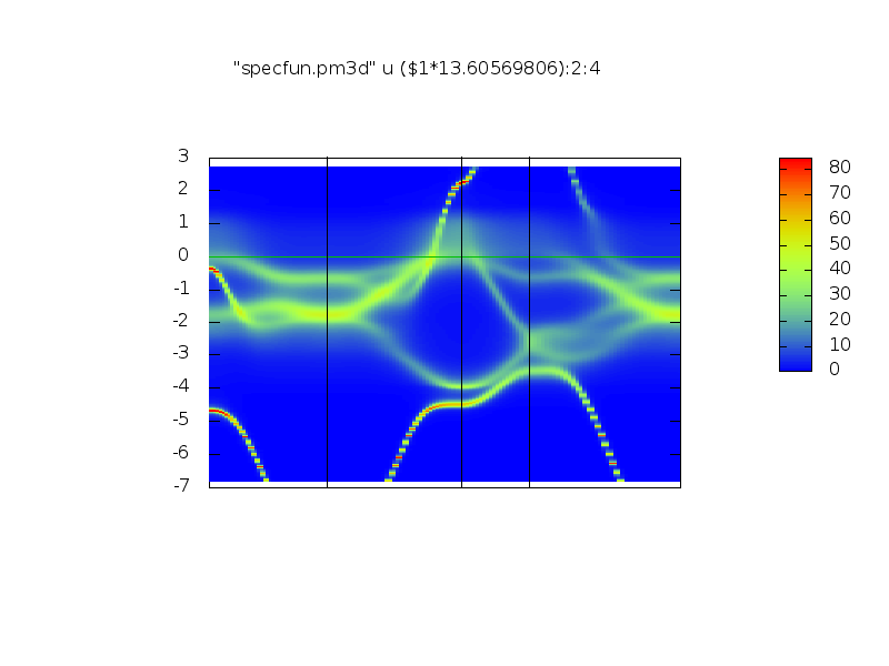
It should create two files: perma_UP.png and perma_DN.png with the spectral funcrions for spin up and down. y-axis is in mRy.

They should look somehow like (up and down):

permaup figure .

permadn figure .

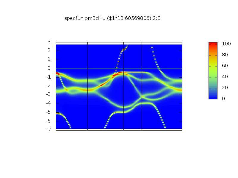Now you can try to run different concentrations of Cu and Fe to see how it affects the spectral functions.

For a detailed analysis of this system, see Reference 1.

Footnotes and references

¹ This tutorial was adapted from the following paper:
The magnetic, electrical and structural properties of copper-permalloy alloys
Makram A. Qader, Alena Vishina, Lei Yu, Cougar Garcia, R. K. Singh, N. D. Rizzo, Mengchu Huang, Ralph Chamberlin, K. D. Belashchenko, Mark van Schilfgaarde, and N. Newman
Journal of Magnetism and Magnetic Materials, Vol. 442, 15.11.2017, p. 45-52.

² I. Turek, V. Drchal, J. Kudrnovsky, M. Sob, P. Weinberger. Electronic structure of disordered alloys, surfaces and interfaces. Kluwer academic publishers (1997), see Eqs. (4.25)-(4.29).

Table of Contents

Preliminaries

Building the ctrl file

Spectral function calculations with lmgf

Plotting the spectral function

Footnotes and references