Tuning CTQMC Parameters for Nickel
Issues with input and parameters
The aim of this tutorial is to give some indications on how to set the parameters of the DMFT calculation. We will give some examples of how the output should look like and, more importantly, how it shouldn’t.
The basic input files for the CTQMC solver are the PARAMS file, the Trans.dat, the actqmc.cix file, the Delta.inp, the Eimp.inp and finally the status files. Moreover lmfdmft requires the indmfl file. Descriptions of how to set the relevant parameters of the PARAMS, and the indmfl files are given below. You are not supposed to edit the other files, so we don’t give an explanation of them here.
Among the output files, the most important ones are Sig.out and histogram.dat. We will refer to these two to judge the quality of our calculation.
Tuning input parameters for CTQMC+DMFT
Here we provide a standard PARAMS file for CT-QMC calculation for Nickel at =50 (eV) which should be run on at least 72 cores to produce high quality data over all energies.
OffDiagonal  real
Sig  Sig.out
Gf  Gf.out
mode GH
svd_lmax 25
Delta  Delta.inp
cix  actqmc.cix
Nmax  3000         # Maximum perturbation order allowed
nom  200          # Number of Matsubara frequency points sampled
exe  ctqmc        # Name of the executable
tsample  50       # How often to record measurements
Ed [ -26.407760, -26.407519, -27.011761, -26.407397, -27.011682, -25.662041, -25.662114, -26.272431, -25.662012, -26.272482] # Ed: Eimp-Edc for PARAMS
M  80000000     # Total number of Monte Carlo steps per core
Ncout  2000000            # How often to print out info
PChangeOrder  0.9         # Ratio between trial steps: add-remove-a-kink / move-a-kink
mu   26.407760 # mu = -Eimp[0] for PARAMS
warmup  5000000           # Warmup number of QMC steps
sderiv  0.02      # Maximum derivative mismatch accepted for tail concatenation
aom  10           # Number of frequency points used to determin the value of sigma at nom
U    4.0
J    0.3
nf0  8.0
beta 50.0
The mode GH in the PARAMS file means that the Green’s functions (G) are sampled on Matsubara frequencies for first 200 frequency points as specified by the tage nom 200 and the high energy tail is corrected by Hubbard solver (H). There are few other options available for the sampling modes like; GM, SH, SM. Here, S stands for self energy sampling and M stands for analytic moment corrections for the high energy tail.
Our experience says that GH is the most stable mode for a very good quality low energy and high energy data. However, these modes don’t solve the problem related to the noise at intermediate frequencies. To address that problem the expansion in SVD basis is introduced by Kristjan Haule. In his own language: CTQMC was substantially reconfigured. The Green’s function or self-energy (or even the two particle vertex) can now be sampled both in the Matsubara frequency (old way) and in more efficient SVD basis ( These are SVD vectors of the analytic continuation kernel). This last method removes all noise at intermediate frequency.
A reasonably well converged dataset for Nickel for single-particle quantities:
Here you can find a very well converged dataset for Nickel for all the single-particle quantities from this link. The calculation converged after 14 iterations with a PARAMS file that look like above. To fasten the calculation what you can do is to add the svd_lmax switch only after 13 iterations, where you reliaze that all the quantities are converged, except for the fact that there is noise at intermediate frequencies. This calculation will run for 7-8 hours on 24 cores. You can, however, reduce the time by increasing the number cores and still acieve similar good statistics.
Impose symmtery
However, if you want to impose symmetries within and sectors respectively, you want to modify the indmfl.ni file.
The indmfl.ni in that case looks like:
0.1 1.2 1 2                # hybridization Emin and Emax, measured from FS, renormalize for interstitials, projection type
1 0.0025 0.0025 600 -3.000000 1.000000  # matsubara, broadening-corr, broadening-noncorr, nomega, omega_min, omega_max (in eV)
1                                     # number of correlated atoms
1     1   0                           # iatom, nL, locrot
  2   2   1                           # L, qsplit, cix
#================ # Siginds and crystal-field transformations for correlated orbitals ================
1     5  2       # Number of independent kcix blocks, max dimension, max num-independent-components
1     5  2       # cix-num, dimension, num-independent-components
#---------------- # Independent components are --------------
'x^2-y^2' 'z^2' 'xz' 'yz' 'xy'
#---------------- # Sigind follows --------------------------
1 0 0 0 0
0 1 0 0 0
0 0 2 0 0
0 0 0 1 0
0 0 0 0 2
#---------------- # Transformation matrix follows -----------
 0.70710679 0.00000000   0.00000000 0.00000000   0.00000000 0.00000000   0.00000000 0.00000000   0.70710679 0.00000000
 0.00000000 0.00000000   0.00000000 0.00000000   1.00000000 0.00000000   0.00000000 0.00000000   0.00000000 0.00000000
 0.00000000 0.00000000   0.70710679 0.00000000   0.00000000 0.00000000  -0.70710679 0.00000000   0.00000000 0.00000000
 0.00000000 0.00000000   0.00000000 0.70710679   0.00000000 0.00000000   0.00000000 0.70710679   0.00000000 0.00000000
-0.70710679 0.00000000   0.00000000 0.00000000   0.00000000 0.00000000   0.00000000 0.00000000   0.70710679 0.00000000
Switches for computing Two-particle Green’s functions
Till this point we have focussed only on the computation of single-particle quantities. However, if we want to compute spin and charge susceptibilities, the first thing we should have is the two-particle Green’s function. CT-QMC allows us to sample to two-particle quantities locally. To do so, we need to add two-switches to the PARAMS file.
SampleVertex 100
nOm 2
SampleVertex 100 implies that a two-particle kink is added (removed) after every 100 kinks for the single-particle Green’s functions. In principle we are free to choose any integer for this particular switch, but 100 or more is recommended lest the computation time explodes. nOm 2 stands for the number of bosonic frequencies on which we want to compute the two-particle Green’s functions. If someone is interested only in the lowest energy excitations for spin and charge, nOm 1 would suffice. However, two-particle Green’s functions are explicit functions of two-fermionic frequencies and one bosonic frequency. If we don’t specify anything in the PARAMS file it is implied that the number of Fermionic frequencies nomv is 50.
The indmfl file
Note: It is planned to change the syntax of this file. It will soon become obsolete!
This file is used by lmfdmft to define which atomic species and orbitals are mapped to the impurity. At the moment the file has a lot of redundant information, reminiscent of the formatting used in K. Haule’s DMFT package. Among all the information reported, you are interested only in a couple of variables at lines three and four.
1                                   # number of correlated atoms
1    1   0                           # iatom, nL, locrot
The first variables defines how many atoms are correlated. Note: At the moment we are testing the code for values higher than 1. So far it hasn’t been possible to treat more than one atom.
The first variable of the second line (iatom=1 in the example) is the index of the correlated atom in the basis chosen. In the example, Ni has only one atom so it’s index is 1. This value has to be consistent with the site.ext file
If the site file is
  ATOM=La         POS=  0.5000000   0.5000000  -0.4807290
  ATOM=La         POS= -0.5000000  -0.5000000   0.4807290
  ATOM=Cu         POS=  0.0000000   0.0000000   0.0000000
  ATOM=O          POS=  0.0000000   0.5000000   0.0000000
  ATOM=O          POS=  0.0000000   0.0000000   0.6320273
  ATOM=O          POS= -0.5000000   0.0000000   0.0000000
  ATOM=O          POS=  0.0000000   0.0000000  -0.6320273
then iatom=3.
All the other values of the file are either ignored or should not be changed.
The PARAMS file
This file is one of the input files read by the CTQMC sovler.
The variables contained in this file define the kind of calculation, allowing for a tuning of the Quantum Monte Carlo algorithm and details on how to treat the connection between the low-energy and the high-energy part of the self-energy. An example of the PARAMS file is reported in a dropdown box of the second tutorial.
Basic parameters (U, J, nf0 and beta)
Among the possible parameters are U and J, defining respectively the Hubbard in-site interaction and the Hund’s coupling constant in eV. Warning: The same value of J has to be passed to atom_d.py as well.
The variable nf0 is the nominal occupancy of the correlated orbitals (e.g. nf0 9 for , nf0 8 for Ni).
Finally beta fixes the inverse temperature in eV.
Warning: Don’t forget to be consistent when you run atom_d.py (which wants J as an input) and lmfdmft (for which the flag --ldadc= has to be consistently defined as U(nf0-0.5)-J(nf0-1)*0.5).
Setting the number of sampled frequencies (nom and nomD)
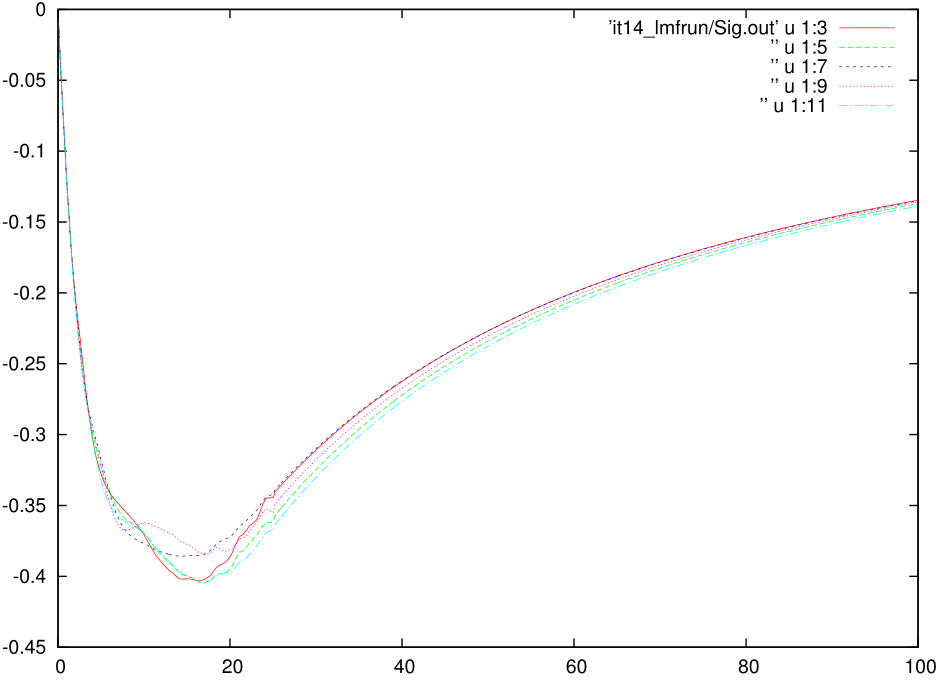
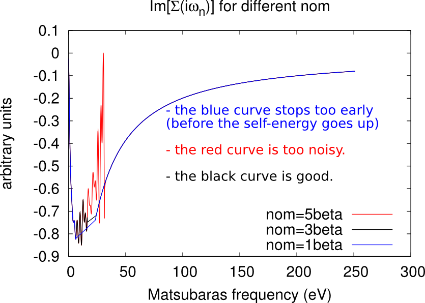
The CTQMC solver gives a very accurate description of the self-energy in the low frequency range (for Matsubara’s frequencies close to 0), but it becomes too noisy at high frequencies.
Let be the total number of Matsubara’s frequencies. This number has been defined through NOMEGA in the ctrl file during the lmfdmft run. Only the first nom frequencies are actually sampled by the CTQMC solver, while the other points are obtained analytically through the approximated Hubbard 1 solver (high-frequency tail).
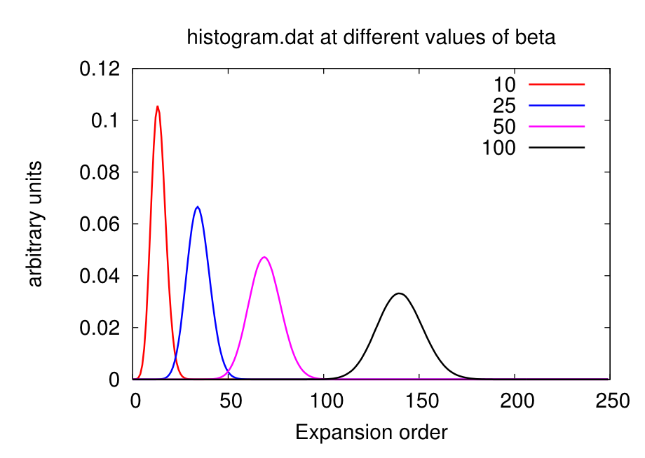
Excessively low values of nom will miss important features of the self-energy (e.g. a convex point in ), while too high values will give excessively noisy results. As a rule-of-thumb, a good initial guess is nom beta, but this value has usually to be adjusted during the DMFT loop. Some examples of how the looks like at different values of nom are given in the figures below.
Setting the number of Monte Carlo steps (M and warmup)
The higher is the number of Monte Carlo steps, the lower the noise in the QMC calculation. The parameter M defines the number of MC steps per core. Reliable calculations easily require at least 500 millions of steps in total. For instance, if you’re running on 10 cores, you can set M 50000000. You can judge the quality of your sampling by looking at the file histogram.dat. The closer it looks to a Gaussian distribution, the better is the sampling.
Warning: The variable M should be set keeping in mind that the higher it is, the longer the calculation. This is crucial when running on public clusters, where the elapsed time is computed per core. Too high values of M may consume your accounted hours very quickly! Moreover remember that you are supposed to broaden the output at each iteration, so you don’t actually need very clean Sig.out.
During the first warmup steps results are not accumulated, as it is normal on Monte Carlo procedures. This gives the ‘time’ to the algorithm to thermalise before the significative sampling. You can set warmup=M/1000.
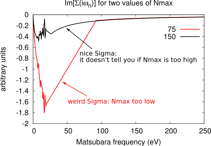
Setting the cutoff expansion order (Nmax)
The variable Nmax defines the highest order accounted for in the hybrdization expansion. If you have chosen an excessively low values of Nmax, the histogram.dat file will be cut and will look weird, as shown below.
You should chose Nmax high enough for the Gaussian distribution of histogram.dat to be comfortably displayed. However note that the higher Nmax the longer the calculation, so chose values just above the higher Guassian tail.
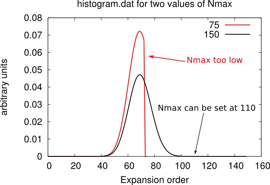
Warning: the value of beta affects the number Nmax, so calculations on the same material at different temperatures will require different Nmax. At low beta, the Gaussian distribution is sharper and centered on lower order terms, as shown below. Therefore lower beta require lower Nmax.
Connecting the tail (sderiv and aom)
The connection between the QMC part and the Hubbard 1 part is done with a straight line starting at frequency number nom+1 and running until it intersect the Hubbard 1 self-energy. You can see it by comparing the Sig.out file with the s_hb1.dat (Hubbrad 1 only).
The two variables controlling the connection are sderiv, which is related to the angle of the straight line, and aom related to its starting point.
The straight line connecting the low- and the high-frequncy region can easily give rise to unwanted kinks. To broaden Sig.out is necessary to smooth these kinks out as well.
Impurity levels (Ed and mu)
The impurity levels reported at the fourth line of Eimp.inp enters in the PARAMS as the variable Ed. The variable mu is set as the first entry of the Ed with opposite sign.
Warning: These two variables change at every iteration so you have to constantly update their value throughout the DMFT loop.
Phase transition boundaries
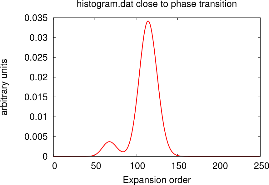
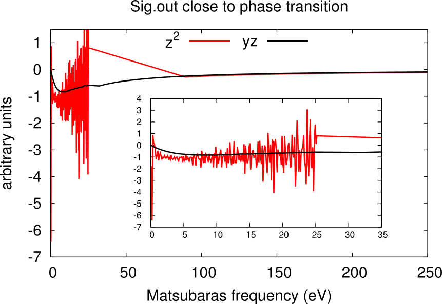
It may happen that, despite the high number of QMC steps, the histogram.dat file displays a double peak distribution simiar to the sum of two Gaussians. This is the case when the material is close to a phase transition.
In this case usually one or more channels of the self-energy are very noisy. One has to run for longer times, or use the status files to restart the calculation many times until only one peaks dominate and the histogram looks like a Gaussian. An example is given in the boxes below.
Using status files
During the calculation, each core generates a status file. They contain some information about the sampling and should be used as restart files for other CTQMC calculations with similar parameters. They are read authomatically if they are in the folder where ctqmc is running.
They can be used basically in two ways.
- If you are performing iteration N, you should copy the status files from iteration N-1 to speed up the convergence of the calculation.
- If you realise that in one ctqmc run, you haven’t achieved a good sampling (e.g. M too low, or close to phase transition), than you can run again the calculation without losing the effort already done. When restarted, the ctqmc solver will automatically read the status files and retrive their information.
Warning: Since there is one status file per core, you must pay attention to run on as many cores as status files you have. It should be safe (but not recommended) to run with a smaller number of cores, while running on more cores than status files gives wrong results.