Configuring lmf and lmgw.sh for HPC architectures

Note this page is under construction

Introduction

Questaal’s codes will use a mix of MPI, OpenMP, and GPU accelerator cards, often in combination, depending on the application. Some of the parallelization is hidden from the user, but some of it requires explicit user input. For heavy calculations special care must be taken to get optimum performance.

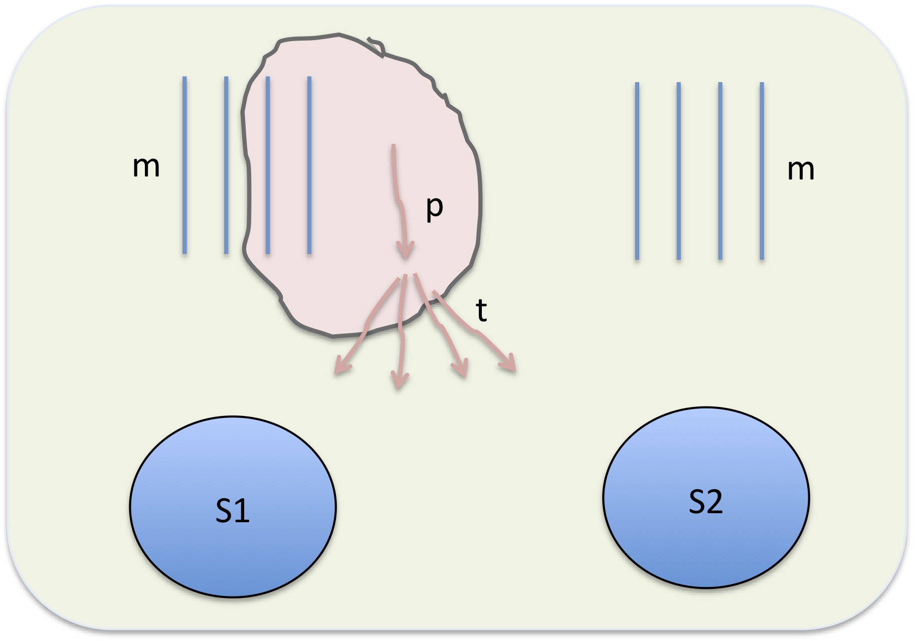
The Figure shows a schematic of a single node on an HPC machine, and processes running on it. Hardware consists of one or more sockets: S1 and S2 are depicted as blue ovals, and memory m as blue lines. Each socket has a fixed number of cores N_c to do the computations. Memory is physically connected to a particular socket.

When a job is launched, it will start a single process in serial mode, or when running MPI, n_p processes where you specify n_p at launch time. A single process (shown as a pink line marked p) is assigned to a core; the process can request some memory, shown as a pink cloud, which may increase or decrease in the course of execution. Since each MPI process is assigned its own memory the total memory consumption scales in proportion to the number of MPI processes. This is a major drawback of MPI: the more processes you run, the less memory available per process. This can be partially mitigated by writing the code with distributed memory: arrays or other data are divided up and a particular process operates mostly on a portion of the entire dataset. When it needs a portion owned by another process, processes can send and receive data via communicators. This exchange is relatively slow, so the less a code reliance on interprocessor communication the more efficiently it executes.

When blocks of code the perform essentially the same function on different data, blocks can be executed in parallel. A single MPI process p can temporarily spawn multiple threads t as shown in the figure— these are subprocesses that share memory. OpenMP executes this way, as do multi-threaded math libraries such as Intel MKL. The big advantage of multi-threading is the shared memory. On the other hand, threads are less versatile than separate processes: OpenMP and multi-threaded libraries are most effective when every thread is doing an essentially similar thing, e.g. running the same loop with different data.

Questaal codes use multiple levels of parallelization MPI as outermost level of parallelization, and multi-threading within each MPI process in critical portions of the code. The multi-threading may be through OpenMP and/or by calling multi-threaded libraries with n_l threads. Since these two kinds of threading are not normally done at the same time, typically you run jobs with n_t=n_l, and this tutorial will assume that to be the case.

You can spread the MPI processes over multiple nodes, which allows more memory to be assigned to a particular process. Thus to run a particular job you must specify:

1. n_n  the number of nodes
2. n_c/n_n  the number of cores/node, which is typically fixed by the hardware and equal to N_c (the number of hardware cores on a node).
3. n_p  the number of processes
4. n_t  the number of threads

You should always take care that n_p×n_t ≤ n_c. This is not a requirement, but running more processes than hardware cores available is very inefficient, since the machine has to constantly swap out processes on one or more cores when executing, which is very inefficient.

Graphical Processing Units (GPUs)

Some of Questaal’s codes (especially the GW suite) can make use of GPU’s. To use them, you typically must specify to the job scheduler some information about them, e.g. how many GPU’s you require. This specification is implementation=dependent, but an example for the Juwels booster is given below. Note that when GPU’s are used, the number of MPI processes should not be very different from the number of GPU’s, depending on the context

Tutorial

Jobs on HPC machines are usually submitted through a batch queuing system. You must create a batch script (usually a bash script) which has embedded in it some extra special instructions to the queuing system scheduler. (How the special instructions are embedded is dependent on the queuing system; a typical one is the slurm system, which interprets lines beginning with #SBATCH as an instruction to the scheduler instead of a comment. Apart from the special instructions, the script is a normal bash script.) These special instructions must specify as a minimum, the number of nodes n_n. You may also have to specify the number of cores n_c although, as noted, it is typically fixed at N_p×n_n. n_p and n_t are specific to an MPI process and are not supplied to the batch scheduler.

The script consists of a sequence of instructions, shell commands such as cp ctrl.cri3 ctrl.x, executables such as lmf ctrl.x or other scripts such as the main GW script, lmgw.sh described below.

An executable may be an MPI job. When launching any job (MPI or serial) you must specify the number of threads n_t. Do this by setting environment variables in your script

OMP_NUM_THREADS=#           ← for OpenMP
MKL_NUM_THREADS=#           ← for the MKL library, if you are using it

Here #=n_t. You also must specify the number of MPI processes, n_p. Usually MPI jobs are launched by mpirun (e.g. mpirun -n # ... where #=n_p), though a particular machine may have its own launcher (for example the juwels supercomputer uses srun).

Note: MPI processes can be distributed over multiple nodes, but there is an associated cost: when data must be distributed between processes or gathered together from multiple processes, the transfer rate is much slower when processes are on different nodes. There is both a latency (time to initiate the process), and a transfer rate. Both are hardware-dependent. Thus it is advisable to put some thought into how many nodes and cores are appropriate for a particular job.

1. lmf with MPI

Questaal’s main one-body code, lmf, will use MPI to parallelize over the irreducible k points. You can run lmf with MPI using any number of processes n_p between 1 and the number of k points n_k. Invoking lmf with n_p > n_k will cause it to abort.

To see how many irreducible k points your setup has, run lmf with --quit=ham and look for a line like this one

 BZMESH: 15 irreducible QP from 100 ( 5 5 4 )  shift= F F F

This setup has 15 irreducible points, so you can run lmf with something like mpirun -n 15 lmf ...

Multithreading within lmf

To also make use of multi-threading, you can set OMP_NUM_THREADS and MKL_NUM_THREADS. As noted earlier, n_p×n_k should not exceed the number of hardware cores you have. Suppose your machine has 32 cores on a node, and you are using one node. Then for the preceding example you can run lmf this way OMP_NUM_THREADS=2 MKL_NUM_THREADS=2 mpirun -n 15 lmf .... Since 2×15 ≤ 32, the total number of threads will not exceed the number of hardware cores. To make it fit well, try to make n_k/n_p not too different from an integer.

lmf has two branches embedded within itself: a “traditional” branch which is comparatively slow but memory efficient, and a fast branch which can be much faster, but consumes a great deal more memory. By default the slow branch executes; to invoke the fast branch, include --v8 on the command line. Both branches use standard BLAS library calls such as zgemm, for which multithreaded versions exist, e.g. MKL. The fast branch also makes of some OpenMP parallelization, and moreover, some of the critical steps (e.g. the FFT, matrix multiply) have been implemented to run on Nvidia V100 and A100 cards as well. With the --v8 switch, GPU’s enhance the performance of lmf immensely. Thus it is very desirable to use the --v8 branch, but there are some limitations. First, the larger memory usage may preclude its use on smaller machines when using it for large unit cells; also some of the functionality of the traditional branch has not yet been ported to the fast branch.

Tips

1. For small and moderately sized cells, MPI parallelization is more efficient than OMP. In this case it is best to distribute the (n_p, n_k) combination heavily in favor of n_p, subject to the restriction n_p ≤ n_k.

2. If you need to save memory, first use BZ_METAL=2 or (if a system with a large density-of-states at the Fermi level) BZ_METAL=3.

3. When using lmf for large cells, it may be necessary to keep the number of processes per node low. This need not be an issue if you have a machine with multiple nodes, as you can use as few as one process per node. For example, a calculation of Cd₃As₂, a system with an 80 atom unit cell and a calculation requiring 8 or more irreducible k points, the following strategy was used.
   • On a single-node machine with 32 cores, BZ_METAL was set to 2 and lmf was run in the traditional mode with
     env OMP_NUM_THREADS=4 MKL_NUM_THREADS=4 mpirun -n 8 lmf ...
   • On the Juwels booster, a many-node machine 48 cores/node, the same calculation was run on 4 nodes with
     env OMP_NUM_THREADS=48 MKL_NUM_THREADS=48 srun -n 4 lmf --v8 ...
4. Forces with --v8. The calculation of forces has not been yet optimized with the --v8 option, and requiring them in that mode can significantly increase the calculation time, particularly if you are using GPUs. If you don’t need forces, set HAM_FORCES=0; if you, set HAM_NFORCE nonzero, e.g. HAM NFORCE=99. Then lmf will make the system self-consistent before calculating the forces, so they are calculated only at the end and the net cost of calculating them is much smaller.

lmf with GPU’s

Some of the critical steps of lmf are implemented for GPU’s. If your job uses them, it is advised that you us an integer multiple of number of GPU’s for the number MPI process, and that integer multiple should be a small integer, like 2 or 4. For large systems, it is advised to use one MPI process/GPU.

2. The lmgw.sh script

Overview

lmgw.sh is a bash script, and is Questaal’s main driver for GW calculations. This page has a user’s guide, including documentation of its command line arguments.

lmgw.sh is designed to run QSGW on HPC machines, as explained in this section.

The QSGW cycle makes a static, nonlocal self-energy Σ⁰. The QSGW cycle actually writes to disk ΔΣ = Σ⁰−V^xc(DFT), so that the band code, lmf, can seamlessly add ΔΣ to the LDA potential, to yield a QSGW potential.

Performing a QSGW calculation on an HPC machine is complicated by the fact that the entire calculation has quite heterogeneous parts, and to run efficiently each of several parts needs to be fed some specific information. lmgw.sh is designed to handle this, but it requires some extra preparation on the user’s part. To make it easier, the GW driver, lmfgwd, has a special mode that automates, or partially automates, the preparatory steps. This will be explained later; for now we outline the logical structure of lmgw.sh and the switches you need to set to make it run efficiently.

lmgw.sh breaks the QSGW cycle into a sequence of steps. The important ones are:

1. lmf  Makes the density self-consistent for a fixed ΔΣ, updating the density from $n$ to $n+{\Delta}n$. (Initially (the “0th” iteration) ΔΣ will be zero.) ${\Delta}n$ modifies V^xc(DFT), so lmf modifies both the Hartree potential and V^xc(DFT). Thus the potential is updated as if the change in Σ from ${\Delta}n$ is given by the corresponding change in V^xc(DFT). In other words, the inverse susceptibility $\chi^{-1} = \delta{V}/\delta{n}$ is adequately described by DFT. As the cycle proceeds to self-consistency change in n becomes small and $\chi^{-1}{\times}\Delta{n}$ becomes negligible, so this assumption is no longer relevant.

2. lmfgwd  is the driver that supplies input from the one-body code (lmf) to the GW cycle.

3. hvccfp0  makes matrix elements of the Hartree potential in the product basis. Note this code is run twice: once for the core and one for the valence.

4. hsfp0_sc  makes matrix elements of exchange potential in the product basis. This capability is also folded into lmsig (next) but the latter code operates only for the valence. hsfp0_sc is run separately for the core states.

5. lmsig  makes valence exchange potential, the RPA polarizability, screened coulomb interaction W, and finally Σ⁰, in a form that can be read by lmf. This is the most demanding step.

Finally there is an optional step that is inserted after making the RPA polarizability.

5a. bse  Add ladder diagrams in the calculation of $W(\omega,q)$. This option is executed when the --bsw switch is used. lmgw.sh synchronizes bse and lmsig.

Running lmgw.sh in a parallel environment

The executables indicated in the previous section have very heterogeneous requirements for parallelization. lmgw.sh can tailor the parallelization for each of the executables described in the previous section, but it takes a fair amount of intervention on the user’s part to tune these flags. Section 3 of this page documents how you can partially automate the setup.

lmgw.sh can be launched in MPI mode with minimum information about how to parallelize, making it easy to set up at the possible expense of larger execution time.

• lmgw.sh in serial mode
  Simply run lmgw.sh without any special instructions for parallelization, as the introductory QSGW tutorial does.

• lmgw.sh in simple parallel mode
  The computationally intensive steps require parallel operation while a number of small steps only run in single process mode. To deal with this disparity and facilitate execution beyond a single node, the simplest option is to launch lmgw.sh with two additional flags, --mpirun-1 "..." and --mpirun-n "..." The former tells lmgw.sh how to execute serial jobs, the latter parallel jobs. For example a command sequence for a calculation on 4 nodes and 32 cores using intelmpi/mpich launchers could be:

  m1="env OMP_NUM_THREADS=32 mpirun -n 1"
  mn="env OMP_NUM_THREADS=16 mpirun -n 8 -ppn 2"
  
  lmgw.sh --mpirun-n "$mn" --mpirun-1 "$m1" ctrl.ext
  

  Remark: how the flags $m1 and $mn must actually be set is machine-dependent. The switches above are representative for a generic intelmpi/mpich launcher.
  Note that the machine will supply 4×32=128 cores, which matches the 16×8 cores $mn is asking for. If the memory allows, you could also use mn="env OMP_NUM_THREADS=8 mpirun -n 16 -ppn 4", which probably runs more efficiently.

As noted, lmgw.sh launches multiple executables, with very heterogeneous requirements for MPI parallelization. Some small steps should be run in serial mode, while others typically in parallel mode. You can specify specific launchers for each of the steps described here.

3. Using lmfgwd to assist in setting up lmgw.sh to run with multiple processors

To run lmgw.sh optimally on an HPC machine, you need to pay attention to the following considerations:

1. Create a batch script. This consists of two parts, as explained in more detail below.
   • instructions to the slurm batch scheduler, e.g. to tell it how many resources you are allocating
   • bash shell commands that set up and run lmgw.sh.

2. Make a pqmap file, whose function is discussed below. This file is not essential as lmgw.sh will execute without it, but a well constructed pqmap can significantly improve the efficiency of execution when generating the self-energy.

lmfgwd has special mode to automatically construct pqmap (an illustration is given in the the Fe tutorial, and there is another in Example 1 below. Also it can be used to partially automate the construction of a batch script. (Making pqmap and making a skeleton batch script are independent of one another.)

A typical command has the structure

lmfgwd [usual command-line arguments] --lmqp~rdgwin --job=0 --batch~np=#[~pqmap@<i>map-args</i>][~nodes=#~<i>batch-args</i>]

np=# specifies the number of MPI processes, and ~nodes=# specifies the number of nodes. You must specify --job=0 (--batch works only for job=0). --lmqp~rdgwin tells lmfgwd to take certain parameters from the GWinput file (rather than the ctrl file). You don’t have to do this, but since the GW codes read data from this file if it is there, your configuration is guaranteed to internally consistent if you include this switch. (If you don’t have a general section in GWinput, it doesn’t matter).

The pqmap portion of --batch supplies the input lmfgwd needs to construct a pqmap file. If you augment the command with @plot (~pqmap → ~pqmap@plot), lmfgwd will make a file plot.pq# together with pqmap (# being np). Then

fplot -f plot.pq#

will make a graphic rendition of the “canvas”, plotting process number and step counter on the ordinate and abscissa. It provides an easy way to visualize what pqmap looks like.

The ~nodes portion of --batch makes a skeleton template for a batch job (file batch). It is not possible to make a generic batch script, because the batch scheduler, batch scripts, and compiler are all system-specific. The batch file is merely a skeleton to make it easier to write the script you will actually need. One thing it does supply are individual launchers for the specific executables lmgw.sh runs. Even these strings (arguments for --cmd-lm, --cmd-gd, --cmd-vc, …) are machine- and compiler- specific, so the contents of batch is only a guide. See this description of how to make a skeleton batch file with lmfgwd.

Note: lmfgwd does not write to pqmap, but instead to pqmap-# where  #  is the number of MPI processes, np. This disambiguates pqmap files for the self-energy maker (which reads pqmap-#) so it reads the file appropriate to the number of processes it uses. Similarly any batch template is written to batch-#.

Organization of the self-energy cycle in a parallel environment

As noted above, and entire QSGW cycle has several one-body steps: a charge self-consistency step (lmf), a driver to make the eigenfunction information for GW (lmfgwd), generation of matrix elements Hartree potential, both core and valence parts (hvccfp0). In the two-body steps, matrix elements of exchange (hsfp0) and correlation (lmsig) are made. lmsig is usually by far the most computationally intensive of all, and the rest of this section focuses on it. Nevertheless each step has own unique requirements, and information must be supplied for each step for lmgw.sh to run efficiently. How to do this will be explained in Section 2.3, along with a procedure to automatically generate the key lines for the batch script.

Medium and large HPC machines have multiple nodes, and Questaal’s QSGW has a multilevel parallelization designed for them. At the outermost level it uses MPI, whose processes can span multiple nodes (see figure above; and within an MPI process it uses multiple threads in several ways, e.g. OMP multithreading within a process at various critical blocks of code. It also uses multithreaded libraries (such as Intel’s MKL library when available) for level 3 BLAS. Also, recent implementations make use Invidia GPU accelerators.

As noted earlier, GW cycle must evaluate both the polarizability and the self-energy at a collection of q points (normally the irreducible q points in the Brillouin zone as needed for self-consistency), and for each q there is a loop over k to make a numerical integration.

The modern GW implementation in Questaal combines the construction of the polarizability P and self-energy Σ into one code, lmsig. This makes it possible to avoid writing W to disk and also to make parts of Σ on the fly without having to have computed all of W(q) first. Also lmsig has reorganized this double loop so that each q-k combination may be done independently --- a great boon for parallel implementations. The [pqmap file] is made only if tag pqmap is present.

The only exception to this is the stage where P must be combined with the bare coulomb interaction v to make the screened one, W. At that point, all the q-k combinations must have been evaluated for a given q. The MPI must perform an expensive ALLREDUCE to collect all the q-k combinations for that q into one process. We will return to this point shortly.

Components of a batch job

A batch script involves two distinct parts:

1. instructions to the batch scheduler that specify the resources you need. Typically this consists of the following:

   • Total number of cores n_c and nodes n_n. Typically you do not specify n_n : it is determined from n_c/N_c where N_c is the number of hardware nodes.

   • Number of GPU’s, if any. It should not exceed the number of GPU’s attached to the nodes you allocate.

   • Number of cores/node, n_c/n_n. You often do not need to specify this because it is fixed by the number of hardware cores/node N_c and in any case should not exceed it.

2. bash shell commands to execute the job (in the present case, lmgw.sh). A job typically requires the following:

   • Number of processes n_p for MPI for the expensive calculation of Σ

   • Number of processes/node n_ppn to assign (which together with n_p specifies the total number of nodes)
      
     The performance of lmgw.sh can also be improved with information for the one-body parts of the cycle, as the optimal distribution of resources is likely different than for the generation of Σ

   • Number of k points lmf requires for Brillouin zone integration

   • Number of q points for which the GW driver lmfgwd makes eigenfunctions

   • Number of q points matrix elements of bare coulomb potential will be evaluated. This will be the number of actual q points + number of offset gamma points.

Information from the last three bullets are needed to make good command-line arguments --cmd-lm, --cmd-gd, --cmd-vc (also corresponding to steps 1,2,3 in an earlier section). Usually you don’t need to specify --cmd-xc, as it will take --mpirun-n in the absence of a particular specification.

3.1 Using lmfgwd to make a skeleton batch script

This section outlines what goes into a script to submit to a queuing system, and also discuss how to configure the lmgw.sh instruction within the script. As noted earlier, lmgw.sh requires several switches to execute efficiently, and configuring these switches can be somewhat involved.

The discussion here is written around the slurm queuing system; other batch schedulers will have similar but distinct instructions. A script that is submitted to the scheduler has the structure of a usual bash script, with instructions to the scheduler folded in. (We are assuming here this script is a bash script.)

Lines beginning with #SBATCH are interpreted as instructions the scheduler, while they are comments to bash itself. #SBATCH instructions usually appear near the top of the script. There are numerous possible instructions, but the key ones are those that allocate resources: number of nodes, possibly number of GPU’s, and execution time. Unfortunately slurm tends to conflate processes (or “tasks”) with resources allocated; it tries to abstract away the number of nodes you need and calculates it internally from other parameters. As a result the resource allocation part is often confusing and more complicated than it need be. Moreover, there some variation in how different implementations of slurm interpret these instructions, so it is difficult to give a uniform prescription.

Moreover, each HPC system has its own implementation of MPI, and once again making instructions that apply to all machines is not feasible or optimal.

Setting the switches by hand is tedious and error-prone, and ideally the construction of this script would be fully automated, it being generated from minimal information you supply. However, these twin issues preclude full automation; but as a workaround, Questaal has a facility that generate key portions of the script, with ability to adapt to a limited number of specific architectures. It is built into lmfgwd and you invoke it as follows

lmfgwd [usual command-line arguments] --lmqp~rdgwin --job=0 --batch~np=#~nodes=#~<i>architecture</i>[~<i>other-tags</i>]

You must specify --job=0 (--batch works only for job=0). --lmqp~rdgwin tells lmfgwd to take certain parameters from the GWinput file, (rather than the ctrl file). You don’t have to do this, but since the GW codes read data from this file, including this switch will make your configuration internally consistent. Particularly relevant are the ones related to the k mesh (e.g. tag n1n2n3 in GWinput).

--batch tells lmfgwd to generate segments of a batch script. --batch accepts several modifiers. The required ones are ~np=#, ~nodes=#, ~architecture. As of this writing, lmfgwd knows about the following architectures.

• a generic vanilla machine. Specify with vanilla# where # is the number of cores/node, viz  --batch~vanilla16 .
• the gravity cluster at King’s College London. It is written for a queuing system configured for hardware consisting of 11 nodes, with each node having 256G RAM and 32 nodes. Specify with --batch~gravity.
• the eagle cluster operated by National Renewable Energy Laboratories. eagle is a moderately large HPC system with about 2600 compute nodes available for HPC jobs, typically with 36 cores/node. It has a modest number of Nvidia V100 GPU accelerators. Specify with --batch~eagle or --batch~eagle~gpu.
• the Juwels supercomputer in Julich, Germany. Juwels is a powerful HPC system, particularly “Booster” cluster with 4 Nvidia A100 cards/node. Specify with --batch~juwels~gpu.
• the tgcc supercomputer in France. tgcc is a CPU-only machine, with a large number of cores. Specify with --batch~tgcc.

Besides supplying #SBATCH instructions for the SLURM scheduler, --batch instruction supplies a template lmgw.sh instruction and shell variables that are fed to it. You can of course set these variables by hand (and may need to do so, depending on your hardware configuration), but except for the hardware noted above, lmfgwd can only generate guesses for strings. On the other hand, setting the switches by hand is tedious and error-prone. You may want to try one of the architectures noted above and amend the strings according to your cluster. --batch makes template shell variables to assign to --mpirun-1, --mpirun-n, --cmd-lm, --cmd-gd, and --cmd-vc etc., in the batch script, and writes these strings to file batch-np.

The --batch mode writes various segments of a template batch script to file batch-np. (np is the number of processes you specify). The primary other function of --batch is to make the pqmap file. Generation of pqmap and batch are independent of each other.

For an example, see this tutorial.

Introduction to pqmap

By far the most costly step lmgw.sh has to execute is the self-energy generator, lmsig. Its efficiency can be greatly improved if you supply a helper file pqmap, as explained here.

lmsig must generate a self-energy Σ(q) for each irreducible q point, and to do so it must perform an internal integration over k. Thus lmsig must generate contributions to Σ(q) at some q for a family of k points. As just noted, Questaal’s traditional GW code calculates the polarizability for each q (requiring an internal numerical integration over k), stores the screened coulomb interaction W(q) on disk, and then makes Σ(q) by a convolution  i ∫ dk G(q-k) W(k)  of G and W, which is done by another numerical integration over k, on a uniform mesh of points.⁽¹⁾ lmsig is more cleverly designed: it makes each k contribution  G(q-k) W(k)  to Σ(q) independently (similarly for the polarizability). By parallelizing the process over qk pairs it can be extremely efficient; however there is the issue of how lmsig best distributes the q-k contributions over processors.

For optimum performance every process should calculate approximately equal numbers of  G(q-k) W(k)  terms. But when the system has symmetry, the question of how to distribute these terms among processes can be a complicated one, since each q point may have a varying number of k points entering into the numerical k integration. Call this number n_q. Indeed the higher the symmetry, with wider the variation in n_q will be. The MPI implementation in lmsig needs this information to be made optimally efficient; this is what file pqmap contains. The structure of pqmap, and a strategies to employ for making it, are given below.

To visualize how pqmap is constructed, represent the total work as a tiling of rectangles on a canvas or a grid, with the cycle or step count i_step ranging on the ordinate between 1 and n_step, and the process number i_p ranging between 1 and n_p on the abscissa n_p being the number of processes you select. The n_q contributions associated with a particular q are kept contiguous on the canvas: point q is assigned a rectangle of area at least n_q. (This is not an essential condition but it improves interprocessor communication.) The trick is to arrange rectangles, corresponding to the “area” n_q of each q point, as densely as possible. Each rectangle can be constructed in different shapes: for example, if a q point has 29 qk combinations, the area must be at least 29. 29×1 is one possibility; so are rectangles of area 30. 30 has prime numbers 2,3,5, so rectangles 15×2, 6×5, 5×6, or 2×15. are all valid choices. Since interprocess communication is relatively costly, the rectangles are ideally as tall and as thin as possible. This is particularly important when MPI has to perform an ALLREDUCE on the n_q points to make the polarizability.

Let n_qk to be the sum ∑n_q of all qk combinations, and n_step be the maximum number of cycles (aka steps) any one process has to perform. In the graphical representation just described, n_step is the height of the canvas and the width is the number of process n_p, which you choose. We want to minimize n_step, but it clearly has a lower bound : n_step  ≥  n_qk / n_p.

You can make pqmap by hand, but it is a tedious process. The GW driver lmfgwd has a special purpose mode designed to make a sensible pqmap for you. Running lmfgwd with -\-batch~pqmap activates this mode, as described in more detail in the next section.

3.2 Construction of pqmap

As noted each q point may have a widely variable of k points needed for the internal k integration when the system has space group symmetry operations. Without this specific information, MPI is likely not to be particularly efficient when evaluating the crucial step 5 (see lmsig above). To make the most efficient MPI implementation, you can supply a helper file pqmap. The structure of this file is most easily visualized in terms of filling a canvas as explained in the previous section. Here we discuss the structure of pqmap in more detail.

For each q, pqmap has a line with the following form:

   <b>offr</b>   <b>offc</b>   <b>nr</b>   <b>nc</b>   <b>iq</b>

iq is the index to the particular q; offr and offc are the offsets to the canvas (the upper left corner of the rectangle). nr and nc are the number of rows and columns (number of steps and processors) this q point will require. nr×nc must be at least as large as n_q.

lmfgwd --job=0 --batch~np=#~pqmap[@options] creates pqmap.# (# is the number of processes n_p) which “tiles” a canvas of area n_step × n_p. It is tiled with rectangles of area n_q and there are as many rectangles as irreducible q points. The rectangle associated with a particular q has area at least n_q and the width nc must not exceed n_p.

lmfgwd uses a complicated algorithm to tile the canvas. Determining the optimal choice of tiling is a difficult proposition: the number of possible combinations grows exponentially with the number of irreducible k points, and moreover, tall, narrow rectangles are preferable to square or short, fat ones. This is because MPI has to perform an ALLREDUCE step when all the information for a given q is collected. Fatter rectangles entail more processes (and possibly more nodes) which puts more demands on interprocessor communication in the ALLREDUCE step.

The algorithm in lmfgwd follows approximately the following guidelines.

1. Make the rectangles as tall as feasible but not exceeding n_step

2. Join the rectangles as compactly as possible

3. After all the q points have been tiled, identify unfilled spaces on the canvas and fill them by enlarging the rectangles.

3.3 Examples of lmfgwd –job=0 –batch

Both lmfgwd and lmchk accept the --batch tag; however there is a difference. lmfgwd knows about the number of k points the various segments lmgw.sh require, and to make pqmap, the number of k points needed to generate Σ(q) for each q, but lmchk does not. Thus, for lmchk to work, you have to supply this information via switches to --batch.

Example 1. InN in the Wurzite structure

This is an example for a hexagonal lattice. The results generated here apply to any hexagonal crystal with 12 space group operations (assuming time reversal symmetry is also allowed).

Paste the box below into init.winn.

HEADER InN in WZ structure
LATTICE
% const a=3.533/.529 q=1.611
  ALAT={a} PLAT= 0.0 -1.0 0.0 sqrt(3)/2 0.5 0.0 0.0 0.0 {q}
SPEC
     ATOM= In   P=0,0,4.9 PZ= 0 0 5.4 LMX=4
     ATOM= N    PZ=3.5 3.5
SITE
     ATOM= In   X=  0.0000000   0.0000000   0.000000
     ATOM=  N   X=  0.0000000   0.0000000   0.619375
     ATOM= In   X=  0.3333333   0.6666667   0.500000
     ATOM=  N   X=  0.3333333   0.6666667   0.119375

Make the ctrl and site files, the atm and basp files, and the GWinput file with the following:

blm --gw --nk=8,8,6 --nkgw=6,6,4 --gmax=9.2 --ctrl=ctrl winn
lmfa --basfile=basp ctrl.winn
lmfgwd winn --job=-1

We will configure this job for the eagle cluster, which has two V100 cards/node. We can run the system with or without GPU’s. It is a small system, so GPU’s are somewhat overkill; all the same we can consider both possibilities.

The first thing is to get a measure of the job’s computational requirements. For this purpose we assume just one MPI process, which we can adjust when we see what the requirements are.

Run lmfgwd in a “test” mode -- without writing any files.

lmfgwd ctrl.winn --lmqp~rdgwin --job=0 --batch~np=1~eagle~noscript~gpu

You should see the following:

expecting for eagle  36 cores/node  2 gpus/node

job has :  40 qp (lmf)  140 qp (lmfgwd)  30 qp (coulomb)  28 qp (sigma)
lmchk --batch~np=1~pqmap@qk=28,84,84,52,84,144,40,28,84,84,52,84,144,40,28,84,84,52,84,144,40,28,84,84,52,84,144,40@plot~eagle~nqlmf=40~nqgwd=140~nqvc=30 ctrl.winn

As of this writing, eagle has 36 cores/node and nodes those with V100 cards have 2 of them. However, these numbers are subject to change as the hardware evolves.

lmf and lmfgwd will evaluate bands for 40 and 140 qp, respectively. Σ will be calculated for 28 qp, and there are 2 additional offset points, so the coulomb interaction is calculated for 30 qp. Also shown (qk=...) are the number of k points at each q. Notice that they are wildly disparate, so a pqmap will be particularly effective. The sum of these numbers is 2064 (shown a few lines earlier in the output), so evaluation of Σ will be parallelized over 2064 combinations.

We now have the parameters we need, and can now use either lmfgwd or lmchk (note the instruction for lmchk above).

<!-- Before doing so, we have to decide on what resources we will use. Consider first the no-GPU case. We randomly pick 2 nodes (somewhat excessive for this small job but useful for demonstration purposes). Since 36 cores are available for one node, we can use 72 cores. These must be distributed between MPI processes and threads. A general rule, OMP starts to lose efficiency when multithreading more than 8, so a good choice would be n_p=9, leaving 8 cores (4/mode) for multithreading. -->

Before doing so, we have to decide on what resources we will use. Consider first the no-GPU case. The 36 cores/node must be distributed between MPI processes and threads. A general rule, OMP starts to lose efficiency when multithreading more than 8, so a good choice might be n_p=9, leaving 4 cores for multithreading if we use only 1 node. We could use 2 nodes but it is somewhat excessive for this small calculation.

Focus first on pqmap. it doesn’t need to know how many nodes will be used, only the number of MPI processes. Cut and paste the lmchk instruction above, replacing np=1 with np=9.

lmchk --batch~np=9~pqmap@qk=28,84,84,52,84,144,40,28,84,84,52,84,144,40,28,84,84,52,84,144,40,28,84,84,52,84,144,40@plot~eagle~nqlmf=40~nqgwd=140~nqvc=30 ctrl.winn

Note the following:

1. The batch mode is designed to make pqmap.# and plot.pq#, and batch-# (# is the number of MPI processes, 9 in this case). lmchk made pqmap.9 and plot.pq9 but aborted without making batch-9 because the number of nodes were not specified. We will do this shortly.

2. You can repeat the command with a different np and compare results. In fact we will want to use np=8, as explained below.

3. The output shows this line:

    makepqmap: filled pqmap for 28 qp  nstep=238 (ideal=230)  nproc=9  nqk=2064  packing fraction 0.9636  avg no proc/q 2.9
   

It says that at least one MPI process will have to go through 238 qk combinations, slightly more than the ideal 230. The map is 96% full, which is quite reasonable since the code executes well below peak performance anyway. You can visualize how the resources are distributed among the individual q-points. Do:

fplot -f plot.pq6
open fplot.ps

Note that the boxes are tall and thin for the most part. This minimizes interprocessor communication. Nevertheless this map is flawed because processes 4,5,6,7 have a big chunk of q-points spread over all of them. It would be better to rearrange the shape of these blocks to make them taller, but the map maker isn’t clever enough for that. It’s better to use np=8 instead. On eagle, lmsig takes 1800 sec to execute using np=9 while only 1300 sec using np=8. Repeat the above lmchk command using np=8.

We are read to make the batch script. Because this is a small calculation we can use just one node. Run lmchk once again, now specifying one node. (Note that you don’t need to make pqmap again though it doesn’t hurt if you do.) One other change: since both lmf and lmfgwd parallelize efficiently over k points (40 for lmf and 140 for lmfgwd), we can increase the number of MPI processes for them with nplm=30~npgwd=35 (or, simpler, nplm=36~npgwd=36).

lmchk --batch~np=8~nodes=1~pqmap@qk=28,84,84,52,84,144,40,28,84,84,52,84,144,40,28,84,84,52,84,144,40,28,84,84,52,84,144,40@plot~eagle~nqlmf=40~nqgwd=140~nqvc=30~nplm=30~npgwd=35 ctrl.winn

Inspect batch-8. It contains lines for most of a complete batch script, though some things are missing (such as setting up modules and the path, and assigning a real execution time). In particular note assignment of variables m1, mn, ml, md, mc.

Next we consider doing the same calculation with GPUs. It makes little sense here because the matrices are too small to take advantage of the immense speedups GPUs can offer on level-3 BLAS operations, but the principles apply to cases where they are useful. There are the following considerations:

• You should not used more than one MPI process per GPU for the time-critical code, lmsig. Since this example has only one node and eagle has 2 GPUs on a node, we will use np=2.
• The one-body codes lmf and lmfgwd are not as well tailored to GPUs yet, and some efficiency can be gained by making the number of processes a small integer multiple of the number of GPUs. Here we will use nplm=6~npgwd=6.

Run lmchk as follows:

lmchk --batch~np=2~gpu~nodes=1~pqmap@qk=28,84,84,52,84,144,40,28,84,84,52,84,144,40,28,84,84,52,84,144,40,28,84,84,52,84,144,40@plot~eagle~nqlmf=40~nqgwd=140~nqvc=30~nplm=6~npgwd=6 ctrl.winn

Compare batch-2 to batch-8 generated previously for the no-GPU job. The differences show what changes that need to be applied to the full batch script. Comparing times: the CPU approach takes about 1700 seconds/QSGW cycle on eagle, while the GPU approach takes about 700 seconds. Nothing to sneeze at, but far from the radical reduction in time seen for larger systems.

Adding ladder diagrams to W

lmgw.sh can also include ladder diagrams via a Bethe-Salpeter equation (bse) to improve the polarizability. When incorporated into the QSGW cycle, it significantly ameliorates the tendency for QSGW to overestimate bandgaps in insulators. This step is very expensive however, and it makes the QSGW cycle much heavier. The following should be taken into account:

• The bse becomes the time- and memory- limiting step
• The two-particle hamiltonian couples every q to every other q. Because of this, taking advantage of symmetry via pqmap are relatively minimal. The bse branch gets mixed up if you try to use it, so be sure to remove pqmap before executing a job with bse.

Here we repeat the preceding calculations but skip generating pqmap, and we will use 4 nodes rather than 1, with 72 MPI processes.

lmchk --batch~bsw~np=72~nodes=4~eagle~nqlmf=40~nqgwd=140~nqvc=30~nplm=40~npgwd=140 ctrl.winn

Note the tag bsw. Compare batch-72 generated just now with the previous batch-8:

diff batch-72 batch-8

This shows what must be changed in the batch script.

References and Other Resources

⁽¹⁾ There is also a convolution over frequency, but lmgw.sh does not try to parallelize the time dimension