Brillouin zone integration
Table of Contents
- Documentation
- Choices in Numerical Integration Methods
- Comparing Sampling to Tetrahedron Integration
- References
This page documents how the Questaal suite performs numerical integrations over the Brillouin zone.
Documentation
Numerical integrations over the Brillouin zone (BZ) occur in several contexts, such as the sum of single particle energies. Care must be taken when performing this integration. In practice the first BZ is divided into a uniform mesh of k-points parallel to the three primitive reciprocal lattice vectors, .
Note: Questaal works with dimensionless reciprocal lattice vectors. , with . ( is the lattice constant in atomic units, read as ALAT in the input file).
The definition of the vectors is standard: construct a 3×3 matrix from the three (dimensionless) primitive lattice vectors (the actual lattice is ). Similarly let be the three vectors composing the 3×3 matrix made from . Then and .
Dividing respectively into sections creates a set of microcells all of the same shape and size. The BZ integration is performed numerically by summing over each of the microcells. You specify through BZ_NKABC. Thus the total number of points in the BZ is . If symmetry operations apply, this number may be reduced.
A uniform mesh is the optimal general purpose quadrature for analytic, periodic functions, in the following sense. Consider the 1D case; the 3D case is exactly analogous. A numerical quadrature from a set of uniformly spaced points integrates exactly any function representable by a Fourier series of Fourier components or fewer, i.e.
for a function periodic in .
Thus when integrating analytic functions, such as the single particle sum for the energy bands of an insulator, the uniform mesh is a good general purpose quadrature. In order to return the discussion to the three dimensional BZ, make the substitution where is a reciprocal lattice vector (some integer multiple of ). The band energy can be represented in a Fourier series
is the analog of ; it is periodic in the vectors. Provided that the Fourier coefficients decay exponentially with , integration with a uniform quadrature converges exponentially with the number of points. does more or less decay this way, typically. In one-band tight-binding theory would correspond to a hopping matrix element separated by distance .
Staggered k mesh
These expressions apply to any uniform mesh, but there is no requirement that the mesh include the origin, . In other words the mesh can be translated by an arbitrary amount in each of the three directions. By default the mesh is selected to include , but there is another natural choice, that applies to each of the three independent vectors : a mesh that contain a point at the origin, or one offset so that points straddle the origin so one point midway between two mesh points falls at the origin. You specify this choice through BZ_BZJOB. Note that BZ_BZJOB is a tag for three numbers, one for each of the primitive reciprocal lattice vectors.
Under what circumstances does this matter? The default and staggered mesh generate different errors, but the errors are of the same order. There no a priori criterion to that will determine in advance which mesh will have the smallest integration error. For band calculations the main reason to choose a staggered mesh is that it may yield fewer irreducible points, even while the total number of points is unchanged. It also may yield more irreducible points. If computation time is an issue, you can check which yields the fewer number of points.
In the somewhat different context of linear response calculations, the response function as is difficult to treat. The GW code has an option to supply a staggered for calculating . Sometimes an offset mesh can significantly improve matters.
One striking example of this is the recently discovered solar cell material, . The figure above shows the static dielectric constant (more precisely ), calculated in the Quasiparticle Self-Consistent GW approximation as a function of n (n = n1 = n2 = n3). The abscissa is scaled so that points are uniformly spaced in 1/n with the origin corresponding to n→∞. Calculations with both the normal mesh (which includes the Γ point) and an offset mesh are shown. Extrapolating either curve to n→∞ results in an estimate for ε∞ of 4.3. Note how much more rapidly converges with the number of k divisions using a staggered mesh.
 )
)See also the description of this figure in the GWinput file documentation.
Note: Meshes generated by BZ_NKABC and BZ_BZJOB are identical to meshes generated by the Monkhorst Pack scheme, with suitably chosen parameters. But Questaal’s specification is simpler and more transparent.
The Single Particle Sum
Numerical integration over the BZ is necessary for band calculations, to obtain charge densities and the sum of single particle energies for total energy. The single-particle sum is the energy-weighted integral of the density-of-states ,
where is the Fermi function. itself is given by a sum over eigenstates as . In a crystal with Bloch states, is a good quantum number we can write it as an integral over the BZ for each band:
When the material is an insulator, sum over occupied states means sum over all the filled bands. Then can be written simply as
Each band is an analytic, periodic function of , so numerical integration on the uniform mesh enables the band sum to converge with the mesh in proportion to how quickly the of the Fourier series above decay.
For a metal the situation is more complicated. There is an abrupt truncation of the occupied part of the band at the Fermi level . At 0K the behavior is non-analytic; at normal finite temperatures the non-analyticity is only a little softened.
Choices in Numerical Integration Methods
The band codes have three integration schemes that determine integration weights for every Quasi-Particle (QP) level at each .
Tetrahedron integration, enhanced by Peter Blöchl’s improved treatment of the Fermi surface [2]. It divides space into tetrahedra (there are 6 tetrahedra for each parallelepiped) and interpolates the energy linearly between the points of the tetrahedron. The Dirac δ-function can be integrated over the tetrahedron by expressing it in the form and approximating by a linear function of k in the tetrahedron.
To use the tetrahedron integration scheme, set BZ_TETRA=t.Gaussian-broadened sampling integration, as extended by Methfessel and Paxton [1]. The basic idea of Gaussian broadening is that a quasiparticle level, which is a -function of the energy in band theory, is smeared out into a Gaussian function. This makes properties analytic again. Methfessel and Paxton extended definition of the -function from the traditional choice of a simple Gaussian of width , to the product a Gaussian and a Hermite polynomial of order 2N. The resulting form of -function has a richer shape: it is still peaked at the quasiparticle level and decays as a Gaussian, but it oscillates as it decays. The generalized Gaussian can rather dramatically improve convergence, as we show below. To use this method, turn off the tetrahedron method (BZ_TETRA=0) and specify and with BZ_N and BZ_W.
Fermi-Dirac-broadened sampling integration. This is similar to Gaussian broadening, but uses the (derivative of) the Fermi distribution for gaussian. It is the physically correct description for finite temperature, but it converges slowly with the k mesh at normal temperatures. To obtain rapidconvergence, artificially high temperatures are often used. To employ FD sampling, turn off the tetrahedron method (BZ_TETRA=0) and set BZ_N=−1. This tells the integrator to broaden the QP level with the (derivative of a) Fermi Dirac function instead of a Gaussian function. Specify the electron temperature through BZ_W (in Ry). For a test case that illustrates Fermi-Dirac sampling, try
fp/test/test.fp coptThere is also a tutorial that uses this method to calculate the specific heat in Al.
Tetrahedron Integration
For self-consistent LDA calculations, Blöchl-enhanced tetrahedron integration is usually the method of choice for small metallic systems. The Figure on the left shows the power of the tetrahedron integration, especially when enhanced with the Blöchl weights. It shows the integration error in the Harris-Foulkes total energy for a fixed density (equivalent to the convergence of the single-particle sum) in MnBi, as a function of the number of divisions. The axis is scaled so that points are uniformly spaced in with the origin corresponding to . MnBi forms in the NiAs structure, which is hexagonal with slightly less than 3/2. Accordingly, the number of divisions along the three directions was chosen to be , for an approximately uniform mesh spacing in the three directions. With Blöchl corrections, the single particle sum is converged to better than 2 μRy at 48 divisions. Without the Blöchl correction term this term convergence is only 100 μRy at 60 divisions. The integration error from the regular tetrahedron method scales as ; the Blöchl correction knocks out the leading term, as is evident from the Figure. For a simple band the scaling improves to .
Band crossing error
There are caveats to keep in mind with respect to this method. Sometimes a pair of bands can cross near . The tetrahedron integrator, which must interpolate a single band between the four corners of a tetrahedron, expects the band to behave in an analytic way. If two bands cross inside the tetrahedron, both the lower band and upper band are non-analytic (in reality both are analytic but the integrator isn’t smart enough to detect that there is a band crossing and switch the levels). When this occurs usually the integrator yields a non-integral number of electrons. It will detect this and print out a warning message:
(warning): non-integral number of electrons --- possible band crossing at E_f
When you get this message usually (not always!) it is because of a band crossing problem. As you proceed to self-consistency it may go away. If not, you need to modify your mesh. The larger the system with a denser mesh of bands, the more serious this issue becomes.
Another drawback with the tetrahedron scheme is that all the eigenvalues must be known before the weight for any one can be determined. This is because integrals are done over tetrahedra, each of which involves four points. Thus unless some trickery is used, two band passes are required: one pass to get all the eigenvalues to determine integration weights, and a second pass to accumulate quantities that depend on eigenfunctions, such as the charge density. The FP code has a “mixed” scheme available: the charge density is calculated by sampling while the band sum is calculated by the tetrahedron method. This avoids a double band pass, and is effective because, thanks to the variational principle, density can be evaluated to less precision than .
Sampling
As the mesh spacing becomes infinitely fine , the quadrature estimate for integrated property of interest (e.g. ) becomes independent of . But with sampling the converged result at the limit is not exact, but depends on : the exact (or 0K) result is obtained only for both and . This should be immediately obvious on physical grounds: the band energy should depend e.g. on temperature.
Thus with sampling there are two independent issues to contend with: how rapidly the result converges with , and the error in the converged result. These issues are not entirely independent: how rapidly the quadrature convergences with also depends on w: the larger w, the more rapid the convergence. This is also easy to understand: the greater the broadening, the smoother and more analytic the behavior at .
The figure above illustrates these points. The BZ integration in the Harris-Foulkes energy is shown for MnBi — the same system used to demonstrate tetrahedron integration. In this figure integrations are carried out with Methfessel-Paxton (MP) sampling described below using =1 for various widths . When is 0.015 (rather large), the energy has converged to within 1μRy of the n→∞ limit for n≥42. But, it converges to a result differing from the exact one by 40μRy. As , ΔE should vanish with n→∞. Indeed this is the case: if =2 mRy the integral is converged to well within 1μRy. But the approach to convergence is much slower: only for n≥90 does the integral stabilize to within 1μRy. The =5 and 10 mRy cases show behavior intermediate between =2 and 15 mRy. The converged integration errors are 2.6μRy and 3.5μRy, respectively.
Methfessel-Paxton sampling
If the -function is broadened with a Gaussian in the standard manner, good results are obtained only when is very small, and the situation would seem to be hopeless. What saves the day is Methfessel and Paxton’s [1] generalization of the broadening function. It starts from the representation of the exact -function as bilinear combinations of Hermite polynomials and a Gaussian
Standard Gaussian broadening represents by the term alone. But by truncating the series at some low order larger than 0, better representations of the -function are possible (figure above) and the integration quality can be dramatically improved. can be well converged without requiring an excessively small .
Choosing any >0 can dramatically improve the quality of sampling integration. The figure above shows how || for MnBi depends on , for a relatively coarse mesh , a very fine one , and intermediate one ( some intermediate ones. For the coarse mesh no advantage is found by varying . This is because the mesh integration error (i.e. the number of in Eq. (2) integrated exactly by the mesh is finite, and essentially equal to ) is larger than the error originating from approximations to the -function.
For the intermediate mesh (n=42) the situation is a bit different. If =0, the approximation to the -function dominates : increasing from 0→1 reduces it by a factor of almost 100! But increasing above 1 has no additional effect: the error remains fixed in the 3-4μRy range. It has already become dominated by the fineness of the -mesh, any adequate (≥1) representation of the -function will serve equally well. Not insignificantly, from the tetrahedron method is in the same range (4μRy).
For the very fine mesh (n=90) much the same story appears, only now that the transition from being dominated by -function error to the discreteness of the mesh doesn’t occur until =4. Because the mesh is so fine, is tiny, of order 0.1μRy.
MP makes it possible to perform quality integrations with sampling. The figure below shows the MnBi test case, now fixing w at 0.015 and varying . (=0 is not shown: is a couple orders of magnitude larger for this w.) In the limit, increasing the polynomial order has an effect somewhat analogous to decreasing . The discrepancy with the exact (0K) result decreases, but the quadrature converges more slowly with n.
There is trade-off: another parameter is available to tinker with. is now a function of an additional variable: . The optimum combination of depends on the precision you need and computer time available. While there is no universal prescription that can be worked out in advance, the following guidelines seem to work fairly well:
- Choose the ratios as closely as possible to the ratios , where the latter are the lengths primitive reciprocal lattice vectors.
- Use at least =1 and unless you are looking for energy resolution (see next section) preferably =3 or 4 with ~0.01. There doesn’t seem to be much downside to using a sizable , but there can be a significant gain.
- If you want very high quality integration, use a fine mesh with ~0.005 and around 3 or 4.
Comparing Sampling to Tetrahedron Integration
Which method should you choose? The answer depends strongly on context.
Response Functions
Consider first the calculation of quantities that involve transitions between two states, such as the joint density-of-states or dielectric function. The Figure below compares Im ε(ω) calculated for Ag, tetrahedron to MP sampling (=1, =0.02). Calculations for 24 and 48 divisions are shown. The sharp shoulder at 0.2 Ry marks the onset of transitions from the Ag d states to conduction band states. This shoulder is seen in experiment, at a slightly higher energy; this is because the LDA puts the Ag d states too shallow.
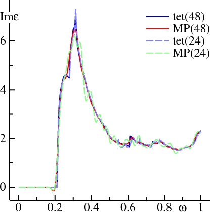
In the tetrahedron case, doubling the mesh affects Im ε(ω) only slightly, showing that it is already well converged at 24 divisions. Sampling with 24 divisions shows Im ε(ω) oscillating around the converged result. With 48 divisions, the oscillations are much weaker, but you can still see Im ε(ω) dip below 0 just before the onset of the shoulder, and round off the first peak around ω=0.28 Ry.
It is possible to get good definition in Im ε(ω) via MP sampling, by increasing N or reducing W, or some judicious combination of the two. However, many more k-points are required. The figure below shows that Im ε(ω), calculated with =1, =.01, can pick up the shoulder at ω=0.28 Ry, but there is ringing around the converged result. This is because oscillates around 0 for ≥1, as seen in the figure for DN(sampling section). Increasing n to 96 divisions yields Im ε(ω) with definition almost as good as the tetrahedron method.
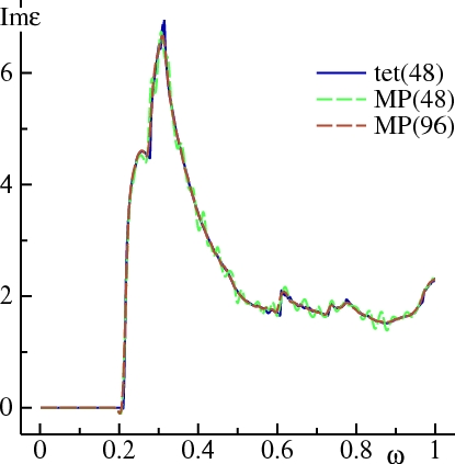
In general, the larger you choose, the better definition you will have if your k mesh is sufficiently fine. But the larger , the more ‘wiggly’ response function will be when you haven’t converged the mesh sufficiently.
Generally speaking, for linear response calculations the tetrahedron method is superior. But, see Note, next.
Note: the existing implementations of tetrahedron may have a problem for tetrahedra that contain multiple bands crossing . We have not fully understood the problem yet, but have discovered that for some metals, (e.g. a four-atom supercell of Ag), a spurious peak in Im ε(ω) can appear for ω→0. A peak actually should exist there, but it originates from the Drude term which is not properly accounted for in this method. So if the peak appears, it does so for spurious reasons.
The Self Consistency Cycle
BZ integration is also required to make the ordinary density-of-states (either total, or resolved by orbital) for the self-consistency cycle or to calculate the single-particle sum for total energy. Here also tetrahedron integration is generally superior, and is usually preferred unless problems arise, e.g. issues with band crossings.
Nevertheless there are circumstances where sampling is a better choice, even apart from the band crossing issue. To calculate the shear modulus of Al, tetrahedron integration requires a very fine mesh. But doing integrations with Fermi Dirac statistics at a rather high temperature, rapidly convergent results can be obtained. To check convergence you can use several temperatures and extrapolate to 0K.
Another example is the magnetic anisotropy. As with the Al shear constant, it is not the absolute value of the energy (mostly single particle sum) that matters, but its variation with some perturbation such as a shear or the addition coupling to the hamiltonian. In such cases the error of the energy difference can be smaller, and more stable, with a suitably chosen sampling method. The table below shows the magnetic anisotropy, in Ry, for CoPt in the L10 structure, using a mesh of 30×30×24 divisions. (A check was made with 40×40×32 divisions using sampling, and essentially the same results were found.) Calculations were carried out in the LDA with both tetrahedron and sampling methods, either by evaluating the change in the Harris-Foulkes total energy, or by calculating the energy through coupling constant integration of . Calculations were both of the non-self-consistent variety (frozen density at some suitable starting point) and also self-consistent. While all the numbers are fairly similar, there is more variation in the tetrahedron results. Note especially the ehf and cc-int columns. They should give the same answer in all cases.
                                                 ehf(tet)   cc-int(tet)  ehf(samp)  cc-int(samp)
non self-consistent, rho from L.S=0             -0.000084   -0.000077   -0.000078   -0.000077
non self-consistent, rho from full L.S || z     -0.000076   -0.000069   -0.000075   -0.000075
self consistent with 8 symmetry operations      -0.000077   -0.000070   -0.000078   -0.000078
self consistent with no symmetry                -0.000078               -0.000077   -0.000076
References
[1] M. Methfessel and A.T. Paxton, Phys. Rev. B, 40, 3616 (1989)
[2] P.E. Blöchl, O. Jepsen and O.K. Andersen, Phys. Rev. B 49, 16223 (1994)