Levenberg-Marquardt fitting of ASA Hamiltonian to QSGW Energy Bands
In this tutorial, the Levenberg-Marquardt capabilities of lm are explained. They are used here to fit the ASA Hamiltonian to QSGW energy bands in cubic CsPbI3 in the cubic and pseudocubic structures.
It starts from the conclusion of the ASA tutorial for CsPbI3, so if you haven’t completed that tutorial, please do it first.
** Cubic structure **
** Pseudocubic structure **
** QSGW **
** Levenberg-Marquardt **
Introduction
The Levenberg-Marquardt algorithm is a method to fit a nonlinear function of multiple1 variables to data. Here the ASA hamiltonian, normally generated ab initio from density-functional theory, is adapted with empirical adjustments to key potential parameters. Adjustments are made by fitting energy bands or partial DOS to a given reference, e.g. from a QSGW result. In its simplest form, the ASA hamiltonian reads
H has indices HRL,R’L’ which labels the basis set according to site and angular momentum. C and Δ are diagonal matrices, i.e. CRL,R’L’ ∝ δRL,R’L’ and ΔRL,R’L’ ∝ δRL,R’L’, and correspond respectively to the band center of gravity and bandwidth in the absence of hybridization with other bands. S=SRL,R’L’ is a structure matrix, which does not depend on potential.
The Levenberg-Marquardt scheme has been implemented in the ASA band program lm In the present implementation, vectors C and Δ can be adjusted to fit some reference bands or partial DOS. The extremely simple and elegant form of H, and its reasonably good accuracy relative to full LDA calculations, makes it an ideal candidate semi-empirical hamiltonian. These degrees of freedom are minimal, and physically transparent. (See here for an interpretation of C and Δ in the language of multiple scattering theory.) For example the LDA+U method amounts to a shift in C (and also extending it from a matrix diagonal in RL to one diagonal in R but not L).
Levenberg-Marquardt (L-M) fitting
The L-M algorithm is a method to fit a nonlinear function of multiple variables to data. The ASA hamiltonian is normally generated from ab initio density-functional theory. Here the ASA hamiltonian is adapted with empirical adjustments to key potential parameters (PP). Adjustments are made by fitting energy bands or partial DOS to a given reference, e.g. from a QSGW result. In its simplest form, the ASA hamiltonian reads where has indices which labels the basis set according to site and angular momentum . and are diagonal matrices, i.e. and , and correspond respectively to the band center of gravity and bandwidth in the absence of hybridization with other bands. is a structure matrix, which does not depend on the potential parameters.
The L-M scheme has been implemented in the ASA band program lm. In the present implementation, the vectors and can be adjusted to fit some reference bands or partial DOS. The extremely simple and elegant form of , and its reasonably good accuracy relative to full LDA calculations, makes it an ideal candidate semi-empirical hamiltonian. The degrees of freedom are minimal, and physically transparent. (See link for an interpretation of and in the language of multiple scattering theory).
For example the LDA+U method amounts to a shift in and also extending from a matrix diagonal in to a matrix diagonal in but not in any more.
Inputs for Levenberg-Marquardt
The L-M scheme in the ASA modifies vectors and (or some subset of all available and ) by trying to minimize some norm, e.g. RMS difference between ASA and reference energy bands.
Once generated and stored, lm can read the modified ’s and ’s, which modifies the ASA-LDA hamiltonian. lm doesn’t read or store the modified and directly, but the shifts in and : these shifts are added to the standard (LDA) parameters. When lm is run in the L-M fit mode, the shifts are written to file vext0.ext.
lm can read shifts from file vext.ext, which has the same structure as vext0.ext. To make lm to read file vext.ext, add the following token to the HAM category in the ctrl file:
HAM RDVEXT=2
The L-M algorithm is designed to minimize the difference between the ASA bands and a reference set, or the difference in the partial DOS relative to a reference set. As part of the definition of the norm, each band or DOS is assigned a particular weight. The fitting algorithm gives you some control over the functional form of the weight; see ITER_FIT_WT below.
Input parameters controlling the L-M fitting are kept in the ITER_FIT tag of the input (ctrl) file. To fit bands use
ITER FIT[MODE=2 ...]
To fit partial DOS use
ITER FIT[MODE=12 ...]
In the former case, you will need some reference bands; in the latter you will need some reference partial DOS. We give an example below for a L-M fitting to a reference band structure.
This is an example of the ITER_FIT tag as it appears in the ctrl file:
ITER FIT[MODE=2 NBFIT=1 81 NBFITF=1 LAM=1 SCL=5 SHFT=1 WT=0,0,.1]
As noted above, ITER_FIT_MODE tells lm what to fit:
| ITER_FIT_MODE (integer) | Fit mode | |
|---|---|---|
| 0 | No fitting | |
| 2 | fit ASA and to bands | |
| 12 | fit to site partial DOS |
The following tokens apply when bands are fit
| ITER_FIT_NBFIT (pair of integers, default = 1 …) | Indices to lowest and highest bands to include in the fit (missing second argument => highest band in basis) |
| ITER_FIT_NBFITF (integer) | Index to the first reference band to be fit. Use it to skip some core levels present in the reference system but not in the ASA. |
The following tokens apply when DOS are fit
| ITER_FIT_NDOS (integer) | Number of energy points to fit DOS |
| ITER_FIT_WG (real) | Broaden calculated DOS with Gaussian, width . Optional 2nd arg specifies different width for reference DOS) |
The remaining tokens apply to either bands or DOS fitting:
| ITER_FIT_EBFIT (pair of real numbers) | Energy range to fit eigenvalues or DOS | |
| ITER_FIT_WT (3 real numbers, default = 0 0 0.1) | Fitting weights of fit bands or DOS to file data | |
| Arg #1 | defines the functional form of the weights. | |
| 0: all points assigned the same weight | ||
| 1: Fermi function : | ||
| 2: Fermi-like gaussian cutoff : | ||
| 3: Exponential weights : | ||
| 4: Gaussian weights : | ||
| Arg #2 | energy shift, denoted in the expressions above | |
| Arg #3 | energy scale, denoted in the expressions above | |
| ITER_FIT_SHFT (integer, default = 0) | adds constant potential shift to align fit with reference bands or DOS | |
| 0 no shift is added | ||
| 1 Align with reference bands or DOS | ||
| 2 Not implemented | ||
| ITER_FIT_LAM (real, default = 1) | Initial value of Levenberg-Marquardt ; see Numerical Recipes | |
| ITER_FIT_SCL (real, default = 5) | Scale factor for Levenberg-Marquardt (cf Numerical Recipes) |
Fitting the ASA PP on QSGW bands for the cubic structure
We now provide an example for fitting the ASA potential parameters onto the band structure of cubic CsPbI calculated with QSGW (results given in paper analyzing the effects of nuclear motion). NOTE that the following calculations are based on Option 2 (Freeze the Pb 6d at a higher linearization energy) described above.
First, create the file with the data given below
Download the reference band file refbnds_cubic_cspbi_GWsc_noSO.txt from here
Then
cp refbnds_cubic_cspbi_GWsc_noSO.txt refbnds.asa
Edit the file ctrl.asa and change
HAM PMIN=-1 # Constrain Pnu > P_free
into
HAM   PMIN=-1                      # Constrain Pnu > P_free
      RDVEXT=2		 	   # Read shifts in C & Delta from vext.* file
and add the line for the L-M fit
ITER FIT[MODE=2 NBFIT=1 47 NBFITF=7 LAM=0.2 SCL=7 SHFT=1 WT=0,.12,.1]
which means that we are going to fit the ASA PP and to the reference band given in the file refbnds.asa, 47 bands will be fitted starting at bands No 7 (in the refbnds.asa file, the 6 first bands contain some core states, i.e. there is at least one dispersionless (flat) band we do not need to consider. All the 47 bands have the some unit weight.
Finally, put the token BZ_INVIT to false in the part of the file ctrl.asa dealing with the Brillouin zone
# Brillouin zone
  nkabc=  {nkabc}                  # 1 to 3 values
  metal=  {met}                    # Management of k-point integration weights in metals
  INVIT=F			   # avoid error in DIAGNO: tinvit cannot find all evecs
The eigenvectors are then not generated by inverse iteration (which is is the default). The inverse iteration method is more efficient than the QL method, but occasionally it fails to find all the vectors. When this happens, the program stops with the message: DIAGNO: tinvit cannot find all evecs. By using INVIT=F, one avoids this problem.
Start the L-M fit by using
lm -vnit=2 ctrl.asa --iactiv=no > out_lm_LMfit.asa
After 2 iterations, the RMS difference between ASA and reference bands slowly converges.
Using
cat out_lm_LMfit.asa | grep RMS
one should get
 LM fit, starting RMS error=0.0876  lambda=0.2
  LMFITMR:  iter 1  old RMS=0.0876  new RMS=0.0443  lambda=0.2
  LMFITMR:  iter 2  old RMS=0.0443  new RMS=0.0208  lambda=0
  LMFITMR:  iter 2  starting RMS=0.0876  final RMS=0.0208  lambda=0
For a good fit to the bands, the final RMS should be of the order of several .
The resulting shifts in ’s and ’s are stored in the file vext0.ext which should read
% contents=2 format=0 nsp=1
PPAR: ASA2
# class         l isp   shft C    shft Delta  frz
   1  Pb        0  1   -0.154751    0.008507  0  0
   1  Pb        1  1    0.009513    0.031511  0  0
   1  Pb        2  1    0.093307    0.058896  0  0
   2  Cs        0  1    0.056289   -0.040845  0  0
   2  Cs        1  1   -0.148698   -0.056874  0  0
   2  Cs        2  1    0.090362   -0.022224  0  0
   3  I         0  1   -0.050322   -0.012000  0  0
   3  I         1  1   -0.102364    0.029521  0  0
   3  I         2  1    0.042320   -0.043010  0  0
   4  E         0  1   -0.006442    0.024363  0  0
   4  E         1  1   -0.044258    0.010160  0  0
   4  E         2  1   -0.008779    0.032196  0  0
   5  E1        0  1    0.014211    0.019634  0  0
   5  E1        1  1    0.063985    0.003896  0  0
   5  E1        2  1   -0.061891    0.005878  0  0
There are two parameters ( and ) to fit for each channel and for each species (Pb,Cs,I,E,E1). This makes a total of 30 parameters to fit, which might appear to be a lot of parameter to fit. There are however some “recipies” that can be used to minimise (and therefore control a bit more) the number of “floating” paramters for the fit.
The ASA PP, and , for the atomic species (Pb,Cs,I) are the most important to get right. The ’s and ’s of the Empty Spheres (E,E1) play also a substantial role but can be subjected to more constraints.
This is done by changing the values in the last two columns (with header frz = freeze) in the file vext.ext.
Changing means that the corresponding (or ) will be kept frozen (unchanged) during the fitting process.
Changing (or to any other negative integer) for different channels and species creates a new subset. Within this subset, the ’s (or ’s) will be modified by the same amount during the fit.
Let’s give a concrete example:
Start by creating the file vext0.asa containing
% contents=2 format=0 nsp=1
PPAR: ASA2
# class         l isp   shft C    shft Delta  frz
   1  Pb        0  1    0.000000    0.000000  0  0
   1  Pb        1  1    0.000000    0.000000  0  0
   1  Pb        2  1    0.000000    0.000000  0  0
   2  Cs        0  1    0.000000    0.000000  0  0
   2  Cs        1  1    0.000000   -0.000000  0  0
   2  Cs        2  1    0.000000    0.000000  0  0
   3  I         0  1    0.000000    0.000000  0  0
   3  I         1  1    0.000000    0.000000  0  0
   3  I         2  1    0.000000    0.000000  0  0
   4  E         0  1    0.000000    0.000000  0  0
   4  E         1  1    0.000000    0.000000  0  0
   4  E         2  1    0.000000    0.000000  0  0
   5  E1        0  1    0.000000    0.000000  0  0
   5  E1        1  1    0.000000    0.000000  0  0
   5  E1        2  1    0.000000    0.000000  0  0
Then
cp vext0.asa vext.asa
and Edit the file vext.asa and modify its contents with
% contents=2 format=0 nsp=1
PPAR: ASA2
# class         l isp   shft C    shft Delta  frz
   1  Pb        0  1    0.000000    0.000000  0  0
   1  Pb        1  1    0.000000    0.000000  0  0
   1  Pb        2  1    0.000000    0.000000  0  0
   2  Cs        0  1    0.000000    0.000000  0  0
   2  Cs        1  1    0.000000   -0.000000  0  0
   2  Cs        2  1    0.000000    0.000000  0  0
   3  I         0  1    0.000000    0.000000  0  0
   3  I         1  1    0.000000    0.000000  0  0
   3  I         2  1    0.000000    0.000000  0  0
   4  E         0  1    0.000000    0.000000  -1  -3
   4  E         1  1    0.000000    0.000000  -1  -3
   4  E         2  1    0.000000    0.000000  -1  -3
   5  E1        0  1    0.000000    0.000000  -2  -4
   5  E1        1  1    0.000000    0.000000  -2  -4
   5  E1        2  1    0.000000    0.000000  -2  -4
This means that the ’s of the channels $l=0,1,2$ for the empty spheres E are not “moving” independently during the fit, but will be modified by the same amount. Similar constraints apply for the ’s of the channels $l=0,1,2$ for the empty spheres E, and for the ’s and the ’s of the empty spheres E1. While the other 18 parameters for the atomic species Pb, Cs, I are free to “move” independently from each other to allow for the best fit.
Now, run
lm -vnit=4 asa --iactiv=no > out_lm_LMfit_step1.asa
then ~~ cat out_lm_LMfit_step1.asa | grep RMS ~~ should read as
 LM fit, starting RMS error=0.0876  lambda=0.2
  LMFITMR:  iter 1  old RMS=0.0876  new RMS=0.0408  lambda=0.2
  LMFITMR:  iter 2  old RMS=0.0408  new RMS=0.0229  lambda=0.0286
  LMFITMR:  iter 3  old RMS=0.0229  new RMS=0.0181  lambda=0.00408
  LMFITMR:  iter 4  old RMS=0.0181  new RMS=0.0171  lambda=0
  LMFITMR:  iter 4  starting RMS=0.0876  final RMS=0.0171  lambda=0
One can start improving the fit by changing the bands weights in the category ITER_FIT.
For that, edit the file ctrl.asa and change ITER_FIT with the following
ITER FIT[MODE=2 NBFIT=1 47 NBFITF=7 LAM=0.2 SCL=7 SHFT=1 WT=1,.12,.1]
Now the bnds weight follows a Fermi function-like distribution, and the bands with energy around and larger than get a smaller weight.
Then (do not forget to use the previously calculated shifts for the ’s and ’s)
cp vext0.asa vext.asa
Before starting the fit, edit file vext.asa and change the line
2 Cs 1 1 -0.196928 -0.085852 0 0
into the following
2 Cs 1 1 -0.303618 -0.024109 0 0
This avoids unnecessary complications in the following.
Then run
lm -vnit=6 cspbi --iactiv=no > out_lm_LMfit_step2.cspbi
After checking
cat out_lm_LMfit_step2.asa | grep RMS
one should get
  LM fit, starting RMS error=0.0184  lambda=0.2
  LMFITMR:  iter 1  old RMS=0.0184  new RMS=0.00540  lambda=0.2
  LMFITMR:  iter 2  old RMS=0.00540  new RMS=0.00281  lambda=0.0286
  LMFITMR:  iter 3  old RMS=0.00281  new RMS=0.00326  lambda=0.00408
  LMFITMR:  iter 4  old RMS=0.00281  new RMS=0.00324  lambda=0.0286
  LMFITMR:  iter 5  old RMS=0.00281  new RMS=0.00297  lambda=0.2
  LMFITMR:  iter 6  old RMS=0.00281  new RMS=0.00289  lambda=0
  LMFITMR:  iter 6  starting RMS=0.0184  final RMS=0.00289  lambda=0
which represents a better fit. The final RMS is around a few .
One can improve further the fit by changing ITER_FIT with the following
ITER FIT[MODE=2 NBFIT=1 47 NBFITF=7 LAM=0.2 SCL=7 SHFT=1 WT=3,.12,.1]
Now, with the exponential form, the bnds weights are mostly concentrated around .
Then run
cp vext0.asa vext.asa
lm -vnit=8 cspbi --iactiv=no > out_lm_LMfit_step2.cspbi
The final RMS should be
  LMFITMR:  iter 8  old RMS=8.51e-4  new RMS=6.60e-4  lambda=0
  LMFITMR:  iter 8  starting RMS=0.00120  final RMS=6.60e-4  lambda=0
and the final file vext0.asa contains
% contents=2 format=0 nsp=1
PPAR: ASA2
# class         l isp   shft C    shft Delta  frz
   1  Pb        0  1   -0.045168   -0.012894  0  0
   1  Pb        1  1    0.019864    0.032718  0  0
   1  Pb        2  1   -0.101022    0.012278  0  0
   2  Cs        0  1    4.663590    1.320703  0  0
   2  Cs        1  1   -0.220486   -0.047131  0  0
   2  Cs        2  1    0.070615   -0.009268  0  0
   3  I         0  1   -0.144494   -0.008486  0  0
   3  I         1  1   -0.174939    0.040949  0  0
   3  I         2  1    0.140586    0.009191  0  0
   4  E         0  1   -0.022964    0.017607 -1 -3
   4  E         1  1   -0.022964    0.017607 -1 -3
   4  E         2  1   -0.022964    0.017607 -1 -3
   5  E1        0  1   -0.018164    0.007317 -2 -4
   5  E1        1  1   -0.018164    0.007317 -2 -4
   5  E1        2  1   -0.018164    0.007317 -2 -4
One can now calculated the ASA band structure including the shifted ’s and ’s and compare it with the band structure calculated with QSGW (which is in the file refbnds.asa ).
For that, run (suppress the line with ITER_FIT in the file ctrl.asa before calculating the bands)
cp vext0.asa vext.asa
lm ctrl.asa -vnit=1 --band~mq~fn=syml
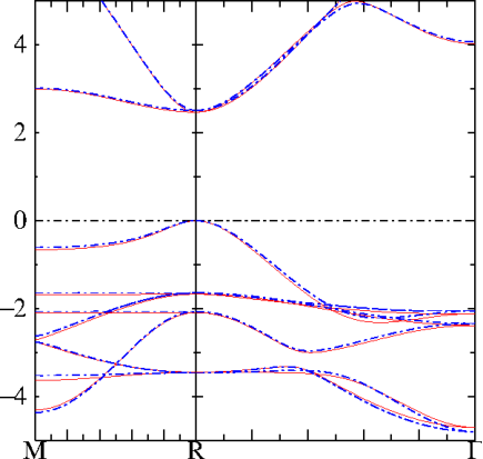
QSGW bands (red) and ASA fitted bands (blue) of cubic CsPbI. That is quite a good fit!
Transferability of the fitted ASA Potential Parameters
… to be continued [27.11.2017]
Footnotes and references
1 The ASA does not keep the density itself, but contracts all the information about the density into energy moments of the sphere charges, , , and , of the density of states for each , and the continuous principal quantum number. . It can do this because of the special structure of the ASA. When the density is needed to make the potential, it is constructed from the and the .
If no data is available for a particular atom, the ASA codes lm, lmgf, and lmpg select from charges in the atom, and sets , and to zero. It takes preset values for the from a lookup table. This is a crude estimate of the density, but it is usually sufficient to make a starting guess, which can be iterated to the self-consistent values.
2 Normally the continuous principal quantum numbers. are allowed to float to band center of gravity (the at which vanishes), but when the partial wave is far removed from the Fermi level, this can cause “ghost bands” to appear. One guard against this is to restrict the , and not let it fall below the free-electron value. Tag HAM_PMIN is designed for this purpose. Another guard is to freeze the to a fixed value, using SPEC_ATOM_IDMOD. Another way is to downfold the . You can tell the ASA codes to downfold a particular state with SPEC_ATOM_IDXDN.