Noncollinear fcc Iron
This tutorial illustrates noncollinear magnetism in lmf, using fcc iron as an example.
Here we take a four-atom supercell of fcc Fe, with lattice vectors in a simple cubic structure. Using the ASA code and spin statics, the stable configuration was found to be one where the spin quantization axis pointed along some permutation of the (1,1,1) direction, so that the angles between each spin are arccos(1/√3), or 109.5o.
The FP code does not as yet implement spin statics, so we take the ASA spin configuration as input.
Setup: files init, eula, ctrl, site, and basp
We will use blm, the input file generator, to build the input file, ctrl.fccfe. Following this tutorial, we build it from an init file specifying structure, in this case a simple cubic cell of Fe with four atoms.
Paste the box below into init.fccfe
HEADER init file for fccfe constructed from questaal test case.
LATTICE
% const a=6.7794173
        ALAT={a}
        PLAT=   1.0000000   0.0000000   0.0000000
                0.0000000   1.0000000   0.0000000
                0.0000000   0.0000000   1.0000000
SPEC
     ATOM=Fe  MMOM=0,0,2
SITE
     ATOM=Fe       POS=    0.0000000   0.0000000   0.0000000
     ATOM=Fe       POS=    0.5000000   0.5000000   0.0000000
     ATOM=Fe       POS=    0.0000000   0.5000000   0.5000000
     ATOM=Fe       POS=    0.5000000   0.0000000   0.5000000
Note there is a species category; this is needed for non-structural information, in this case the initial trial Fe magnetic moment (2 μB on the d orbital).
We also need to specify the Euler angles. The following specifies Euler angles for each site. The lmchk instruction below shows that they point along permutations of [1,1,1] directions, with 109.5o between spins. Paste the box below into eula.fccfe.
    pi/4  acos(1/sqrt(3))     -pi/4
 -3*pi/4  acos(1/sqrt(3))     3*pi/4
  3*pi/4  pi-acos(1/sqrt(3)) -3*pi/4
   -pi/4  pi-acos(1/sqrt(3))   pi/4
Make the ctrl file (input file).
blm --brief --mag~nc~spinor=3 --forces=0 --autobas~ehmx=-.4~eloc=-4.5~loc=5 '--mix~nit=30~mixp=b4,b={beta},k=7' --nk~10 --gw~nk=8 fccfe
This instruction makes the main input file, ctrl.fccfe; the site file specifying structure, site.fccfe; and finally basp.fccfe, the file defining the basis set.
Command-line switches for blm are documented on this page. Specifically:
- –brief : A moderately simple ctrl file, but one with embedded variables to enable command line control of some of the input.
- –mag~nc~spinor=3 : Calculation is to be magnetic and noncollinear.
- –forces=0 : No forces are to be calculated
- –autobas~ehmx=-.4~eloc=-4.5~loc=5 : Sets the basis set.
This switch makes up the semicore 3p local orbital, included as a valence state (not needed, but the calculation is more accurate). - ’–mix~nit=30~mixp=b6,b={beta},w=1,1,wnc=.1,k=6,n=6’ : String for the ITER_MIX tag that controls how the density is mixed.
This exercise does not converge well if blm’s default parameters are used. (This is taken up below.) - –nk~8 : Sets the number of k divisions (8×8×8 k mesh). If you want the calculation to run more quickly, you can reduce the the mesh
- –gw~nk=8 : Enables the ctrl file for a GW calculation. This tutorial doesn’t carry out GW calculations, but the switch enlarges the basis set.
The Fe moment can very sensitive to details.
It turns out that this configuration is consistent with the inversion operation. blm is not capable of determined symmetry operations for noncollinear cases, so we add it by hand. Do the following
sed -i.bak s/'#symgrp spglib'/'symgrp i'/ ctrl.fccfe
To confirm that Euler angles in file eula.fccfe orient spins along the [1,1,1] directions, do the following:
lmchk --euler ctrl.fccfe
You should see that the spin quantization axis points along one permutation of [±0.577350, ±0.577350, ±0.577350].
This table should also be recorded in stdout. It shows that the angles between spins are 109.5o :
          1       2       3       4
       -----------------------------------
    1   --     109.47  109.47  109.47
    2  109.47   --     109.47  109.47
    3  109.47  109.47   --     109.47
    4  109.47  109.47  109.47   --
Self-consistency
The noncollinear calculation proceeds in the same way as a collinear one. First make the atomic densities to be used as a trial starting point for the self-consistency cycle
lmfa ctrl.fccfe
This calculation is too heavy for a scalar job, so you will want to use MPI. Assign variable mn to the MPI instruction, e.g. for a machine with 16 processors,
mn='mpirun -n 16'
Make this system (partially) self-consistent
rm -r mixm.fccfe      ! only needed if restarting a calculation
$mn lmf --rs=0 fccfe > llmf
The ctrl is built to iterate to a maximum 30 iterations. Confirm that the density is reasonably self-consistent:
grep DQ llmf
You should see something like this:
 mixrho:  sought 4 iter, 11362 elts from file mixm; read 0.  RMS DQ=4.46e-2
 mixrho:  sought 4 iter, 11362 elts from file mixm; read 1.  RMS DQ=3.66e-2  last it=4.46e-2
 mixrho:  sought 4 iter, 11362 elts from file mixm; read 2.  RMS DQ=1.01e-2  last it=3.66e-2
 mixrho:  sought 4 iter, 11362 elts from file mixm; read 3.  RMS DQ=3.06e-3  last it=1.01e-2
 mixrho:  sought 4 iter, 11362 elts from file mixm; read 4.  RMS DQ=3.66e-3  last it=3.06e-3
 mixrho:  sought 4 iter, 11362 elts from file mixm; read 5.  RMS DQ=2.18e-3  last it=3.66e-3
 mixrho:  sought 4 iter, 11362 elts from file mixm; read 5.  RMS DQ=1.32e-3  last it=2.18e-3
 mixrho:  sought 4 iter, 11362 elts from file mixm; read 0.  RMS DQ=4.18e-3  last it=1.32e-3
 mixrho:  sought 4 iter, 11362 elts from file mixm; read 1.  RMS DQ=1.72e-2  last it=4.18e-3
 mixrho:  sought 4 iter, 11362 elts from file mixm; read 2.  RMS DQ=7.84e-4  last it=1.72e-2
 mixrho:  sought 4 iter, 11362 elts from file mixm; read 3.  RMS DQ=2.19e-3  last it=7.84e-4
 mixrho:  sought 4 iter, 11362 elts from file mixm; read 4.  RMS DQ=6.04e-4  last it=2.19e-3
 mixrho:  sought 4 iter, 11362 elts from file mixm; read 5.  RMS DQ=6.22e-4  last it=6.04e-4
 mixrho:  sought 4 iter, 11362 elts from file mixm; read 5.  RMS DQ=6.91e-4  last it=6.22e-4
 mixrho:  sought 4 iter, 11362 elts from file mixm; read 0.  RMS DQ=6.23e-4  last it=6.91e-4
 mixrho:  sought 4 iter, 11362 elts from file mixm; read 1.  RMS DQ=1.02e-3  last it=6.23e-4
 mixrho:  sought 4 iter, 11362 elts from file mixm; read 2.  RMS DQ=6.61e-4  last it=1.02e-3
 mixrho:  sought 4 iter, 11362 elts from file mixm; read 3.  RMS DQ=7.26e-4  last it=6.61e-4
 mixrho:  sought 4 iter, 11362 elts from file mixm; read 4.  RMS DQ=7.35e-4  last it=7.26e-4
 mixrho:  sought 4 iter, 11362 elts from file mixm; read 5.  RMS DQ=6.33e-4  last it=7.35e-4
 mixrho:  sought 4 iter, 11362 elts from file mixm; read 5.  RMS DQ=7.24e-4  last it=6.33e-4
 mixrho:  sought 4 iter, 11362 elts from file mixm; read 0.  RMS DQ=6.63e-4  last it=7.24e-4
 mixrho:  sought 4 iter, 11362 elts from file mixm; read 1.  RMS DQ=9.41e-4  last it=6.63e-4
 mixrho:  sought 4 iter, 11362 elts from file mixm; read 2.  RMS DQ=6.63e-4  last it=9.41e-4
 mixrho:  sought 4 iter, 11362 elts from file mixm; read 3.  RMS DQ=7.21e-4  last it=6.63e-4
 mixrho:  sought 4 iter, 11362 elts from file mixm; read 4.  RMS DQ=8.15e-4  last it=7.21e-4
 mixrho:  sought 4 iter, 11362 elts from file mixm; read 5.  RMS DQ=6.41e-4  last it=8.15e-4
 mixrho:  sought 4 iter, 11362 elts from file mixm; read 5.  RMS DQ=7.73e-4  last it=6.41e-4
 mixrho:  sought 4 iter, 11362 elts from file mixm; read 0.  RMS DQ=6.42e-4  last it=7.73e-4
 mixrho:  sought 4 iter, 11362 elts from file mixm; read 1.  RMS DQ=7.37e-4  last it=6.42e-4
The density is very difficult to fully stabilize in this system (see Exercise 3), but the density after the 30th iteration is sufficient to yield observables close to the fully self-consistent ones.
It is also interesting to see what the local moments are. Do the following:
tail -30 llmf
You should see something close to the following
 Sphere charges and magnetization
   ib          q           M           Mx         My         Mz
    1   in   13.217574   1.610001    0.929165  -0.929928   0.929510
       out   13.210675   1.607417    0.927289  -0.928545   0.928293
      diff   -0.006899  -0.002584   -0.001876   0.001383  -0.001217
       mix   13.217512   1.609916    0.929103  -0.929883   0.929470
    2   in   13.217511   1.608115   -0.928273   0.928639   0.928424
       out   13.220771   1.599832   -0.922831   0.924235   0.923925
      diff    0.003260  -0.008282    0.005442  -0.004404  -0.004500
       mix   13.217554   1.607842   -0.928094   0.928494   0.928277
    3   in   13.217173   1.612026   -0.930401  -0.930901  -0.930809
       out   13.228074   1.598908   -0.922526  -0.923701  -0.923163
      diff    0.010901  -0.013118    0.007875   0.007200   0.007646
       mix   13.217295   1.611594   -0.930142  -0.930664  -0.930558
    4   in   13.217435   1.611504    0.930044   0.930530  -0.930633
       out   13.212109   1.607896    0.927773   0.928897  -0.928287
      diff   -0.005327  -0.003608   -0.002271  -0.001633   0.002346
       mix   13.217389   1.611386    0.929969   0.930476  -0.930556
     -----
     total   52.869750   6.440738    0.000837  -0.001576  -0.003367
The local Fe moment is about 1.6μB, somewhat smaller than 2.2μB found in bcc Fe. Note that they point (nearly) along the spin quantization axis.
Energy bands with spin texture
To plot bands on the specified lines, create a symmetry lines file. You can do this by hand, or let lmchk create one for you. We have a simple cubic lattice, i.e. bcc Fe in a four-atom supercell. However, the underlying lattice is bcc, let’s make symmetry lines for it, keeping in mind that four k points in the bcc Brillouin zone will be folded into a single k point.
lmchk ctrl.fccfe --syml~n=50~lblq:G=0,0,0,L=1/2,1/2,1/2,X=1,0,0,W=1,1/2,0,K=3/4,3/4,0~lbl=LGXWGK
Create the bands using generating color weights with spin texture. The following will generate four color weights, projecting the charge and three components of spin onto the Fe d orbitals
$mn lmf fccfe --band@scolst~z=26~l=d@fn=syml
This creates an energy bands file, bnds.fccfe, in an old fashioned format. Inspect the first line of the file. You should see something close to
264 0.00045 4 spin-texture lbl=LGXWGK col1=5:9,21:25,29:33,38:42,54:58,62:66,71:75,87:91,95:99,104:108,120:124,128:132 col2= col3= col4=
This line tells you that the basis consists of 264 orbitals, with 4 color weights corresponding to spin texture. The color weights correspond to projections onto d orbitals, with charge, and the three vector components of the magnetization.
One way to view the spin texture is to use the colors to depict projections onto x, y, and z. In the following instruction spin projections are depicted as three colors (black=, red=, green=), similar to the example for Co in the plbnds documentation.
Do the following
plbnds -range=-9,5,5,10 -wscl=.6,.6 -fplot~sh~ext=z~lt=1,col=0,0,0,colw=1,0,0,colw2=0,1,0~spintexture -ef=0 -scl=13.6 bnds.fccfe
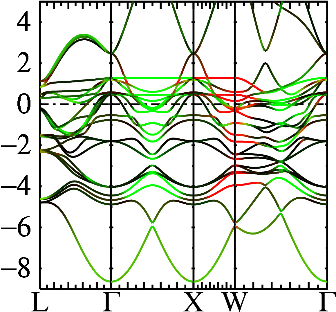
This instruction creates a file fplot.ps, which you can view with your favorite postscript viewer. You should see something similar to the following. (Note that the Γ and X points are identical because of zone folding.)
You can see how the spin quantization axis evolves with k. Particularly interesting are points where the color changes abruptly (see for example midway between L and X at −6 eV), or where two bands of different texture cross.
Fermi surface with spin texture
This section shows how to draw the Fermi surface using colors to reveal the evolution of spin texture.
lmf can create a file with selected bands plotted on a regular 2D mesh (--band option in mesh mode). Data on a regular mesh is the input needed to draw 2D contour plots of constant energy, which if chosen as the Fermi level, is the Fermi surface. This tutorial shows how to use the 2D mesh mode of lmf with fplot to make a figure with a Fermi surface.
To get started, you need to specify an area (square, rectangle, or parallelepiped) lying on a plane in the Brillouin zone), the number of divisions on each axis, and know specify which bands to store.
For the latter, 48 bands lie strictly below the Fermi surface in this system, and the next 12 cross it at some point. To see this run lmf with --minmax :
$mn lmf fccfe -vnit=1 --rs=1,0 --minmax:ef0
--minmax:ef0 causes lmf to display a table with largest and smallest eigenvalues in each band, shifted to align the Fermi level with 0. Thus any band where the maximum value is less than 0, or the minimum value is greater than 0, does not cross the Fermi level. You should find a table something like this
 Lowest, highest evals by resolved band, spin 1, ef shifted to 0 Ry
   1  -3.9578 -3.9532  |   89   1.0628  1.7466  |  177   4.2055  4.8588
  47  -0.1440 -0.0399  |  135   2.8685  3.4373  |  223   6.1189  6.7170
  48  -0.1440 -0.0397  |  136   2.8685  3.4373  |  224   6.1191  6.7188
  49  -0.1327  0.0344  |  137   2.9664  3.4373  |  225   6.3931  7.3532
  50  -0.1326  0.0345  |  138   2.9665  3.4373  |  226   6.3945  7.3538
  51  -0.1325  0.0346  |  139   2.9749  3.4726  |  227   6.3947  7.3556
  52  -0.1324  0.0347  |  140   2.9749  3.4727  |  228   6.3953  7.3560
  53  -0.0890  0.0347  |  141   3.1198  3.6165  |  229   6.4532  7.4404
  54  -0.0890  0.0349  |  142   3.1198  3.6166  |  230   6.4541  7.4432
  55  -0.0815  0.0386  |  143   3.1202  3.6166  |  231   6.7443  7.5163
  56  -0.0815  0.0389  |  144   3.1202  3.6166  |  232   6.7450  7.5182
  57  -0.0135  0.0426  |  145   3.2639  3.6167  |  233   6.7551  7.7141
  58  -0.0135  0.0427  |  146   3.2640  3.6168  |  234   6.7562  7.7153
  59  -0.0133  0.0878  |  147   3.2654  3.6386  |  235   6.9025  7.7166
  60  -0.0133  0.0878  |  148   3.2656  3.6387  |  236   6.9054  7.7182
  61   0.0051  0.0951  |  149   3.3522  3.6387  |  237   7.0465  7.8693
...
Bands 49:60 cross EF.
The --band switch in mesh mode requires an input file defining the mesh (syntax is described on this page). We will choose a square with the Γ point at the center, abscissa along x and ordinate along y, dividing each axis into 35 mesh points (more mesh points gives better definition to the figure).
Paste the box below into file fs.fccfe:
# vx    range   n     vy    range     n  height  band
1 0 0   -.5 .5  35  0 1 0   -.5 .5    35  0.00   49:60
Generate the bands in mesh mode, specifying spin texture for color weights:
$mn lmf fccfe --band~con~scolst@atom=fe@l=2~fn=fs
Inspect the contents of bnds.fccfe. You should see a sequence of 2D arrays in the standard Questaal format for 2D arrays, stacked one after another. There are 60 such data sets: the first 12 are energy bands 49:60 on a 35×35 mesh. The next 12 are weights for the charge density; the next 12 are weights for the x component of magnetization, then y component, then z component.
You can use any facility to draw the Fermi surface. Here we use the contour mode facility in fplot. For each band, fplot will require 4 files: one for the eigenvalues, and three for x, y, z components of the magnetization.
To simplify matters, we will extract the bands and shift them by the Fermi level, to put it at zero. Extract the Fermi level with this
grep efermi= bnds.fccfe | head -1 | vextract . efermi
You could see something similar to 0.001066, which we will use for the Fermi level.
Here we will used the mcx calculator to read bnds.fccfe for each of 12 data sets, containing eigenvalues and write them into files 49, 50, …, 60. Also we will write weights into files x49, x50, …, x60, y49, y50, …, y60, z49, z50, …, z60, for x, y, z components of the the weights.
Set the following shell variables:
rf="-r:open -qr bnds.fccfe -shft=-0.001066"
rfw="-r:open -qr bnds.fccfe"
and run mcx as follows:
mcx [ i=49:60 -qr $rf -w \{i} ] [ i=49:60 -qr $rfw ] [ i=49:60 -qr $rfw -abs -s5 -w x\{i} ] [ i=49:60 -qr $rfw -abs -s5 -w y\{i} ] [ i=49:60 -qr $rfw -abs -w z\{i} ] -show
This should create 60 files, named as described above.
Finally we need an fplot script to draw the figure. Paste the box below into plot.fs :
fplot -frme 0,1,0,1  -x -.5,.5 -y -.5,.5 -tmx .1
   -lt 1,bold=4 -con~colwt=1,0,0~wtfn=x49~colw2=0,1,0~wtf2=y49~colw3=0,0,1~wtf3=z49 -0.00 49
   -lt 1,bold=4 -con~colwt=1,0,0~wtfn=x50~colw2=0,1,0~wtf2=y50~colw3=0,0,1~wtf3=z50 -0.00 50
   -lt 1,bold=4 -con~colwt=1,0,0~wtfn=x51~colw2=0,1,0~wtf2=y51~colw3=0,0,1~wtf3=z51 -0.00 51
   -lt 1,bold=4 -con~colwt=1,0,0~wtfn=x52~colw2=0,1,0~wtf2=y52~colw3=0,0,1~wtf3=z52 -0.00 52
   -lt 1,bold=4 -con~colwt=1,0,0~wtfn=x53~colw2=0,1,0~wtf2=y53~colw3=0,0,1~wtf3=z53 -0.00 53
   -lt 1,bold=4 -con~colwt=1,0,0~wtfn=x54~colw2=0,1,0~wtf2=y54~colw3=0,0,1~wtf3=z54 -0.00 54
   -lt 1,bold=4 -con~colwt=1,0,0~wtfn=x55~colw2=0,1,0~wtf2=y55~colw3=0,0,1~wtf3=z55 -0.00 55
   -lt 1,bold=4 -con~colwt=1,0,0~wtfn=x56~colw2=0,1,0~wtf2=y56~colw3=0,0,1~wtf3=z56 -0.00 56
   -lt 1,bold=4 -con~colwt=1,0,0~wtfn=x57~colw2=0,1,0~wtf2=y57~colw3=0,0,1~wtf3=z57 -0.00 57
   -lt 1,bold=4 -con~colwt=1,0,0~wtfn=x58~colw2=0,1,0~wtf2=y58~colw3=0,0,1~wtf3=z58 -0.00 58
   -lt 1,bold=4 -con~colwt=1,0,0~wtfn=x59~colw2=0,1,0~wtf2=y59~colw3=0,0,1~wtf3=z59 -0.00 59
   -lt 1,bold=4 -con~colwt=1,0,0~wtfn=x60~colw2=0,1,0~wtf2=y60~colw3=0,1,0~wtf3=z60 -0.00 60
This script draws 12 contour plots for contours at zero energy, one for each band, with three weights
Invoke fplot with
fplot -f plot.fs
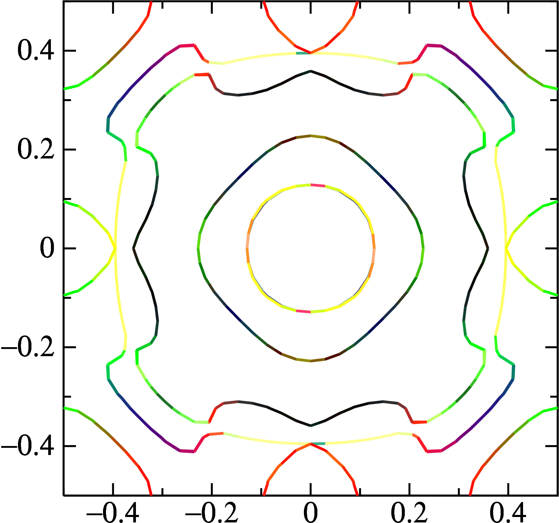
the instruction should create a file fplot.ps, which you can view with your favorite postscript viewer. you should see something similar to the following. red, green, blue correspond to spin oriented along x, y, z, and yellow is a combination of x and y.
it is interesting to see where bands nearly cross (e.g. around (0.2, 0.3)) and the spin quantization axis abruptly changes around the crossing point.
Four component density-of-states
in the noncollinear case, densities have 3 magnetization components as well as the charge component. questaal’s mulliken analysis facility enables you to generate the partial dos including all four compoenents, as explained here.
in lmf, weights needed for mulliken analysis are generated by invoking lmf with the –mull switch. include this switch in the usual way as explained in this tutorial but add ~spinor to the –mull instruction, e.g.:
$mn lmf fccfe --mull~spinor
as written this will generate weights for dos resolved by site, and four channels for each site. lmdos is the postprocessing step, which reads weights generated by lmf and translates them into dos. supply information about the energy window and mesh you want the dos to range over with the –dos, e.g.
lmdos fccfe --mull~spinor --dos:npts=501:window=-1,0.5:h5
this instruction tells lmdos to write the dos to dos.h5. inspect the contents of dos.h5:
h5ls dos.h5
You should see:
h5ls dos.h5
dos                      Dataset {4, 4, 501}
ef                       Dataset {1}
freq                     Dataset {501}
idos                     Dataset {1}
nchan                    Dataset {1}
ndos                     Dataset {1}
nkabc                    Dataset {3}
nkp                      Dataset {1}
nspin                    Dataset {1}
The DOS are stored as element ‘dos’; there are 501 mesh points, 4 channels per site, and 4 sites for which partial DOS are decomposed. (h5ls orders the array indices in reverse order from the way Questaal uses them.) Channel 1 corresponds to charge (which must be always positive definite), channels 2,3,4 to three components x, y, z of the magnetization whose sign may change whether the DOS points along the positive or negative axis.
It is up to you how to make use of the data. Here we use Questaal’s tools to generate an ASCII file containing frequency in the first column and DOS for the first site in the next four columns
mcx -r:h5:id=freq dos.h5 -r:h5:id=dos:c=0,0,1 dos.h5 -ccat > dos.txt
Create a postscript file showing the four DOS:
fplot -coll 2:5 dos.txt

You should see a figure like the one shown. Black is the proper (charge) DOS; red, green and blue show the spin DOS along x, y, z. They are all very similar, except that the DOS along y is the opposite sign (and would flip if DOS were projected along −y). Note that the direction of the magnetization between −0.2 Ry and −0.4 Ry is largely Fe t2g character while the states near the Fermi level are predominantly of eg character. These states are apparently magnetized in opposite directions.
Additional Exercises
Shifting the Fermi level slightly radically alters the Fermi surface. Try modifying the energy in script plot.fs a little (say from (-0.00 to -0.01) see how the Fermi surface changes.
You can confirm that the noncollinear total energy is deeper than the collinear one. To see this, remove eula.fccfe and repeat the self-consistent calculation. You should see that the collinear case is less bound.
Getting the density to go fully self-consistent is exceedingly difficult. You can do it with some special mixing modes. One way accomplish this is to perform iterations in two steps. In the first, modify the mixing mode so that it mixes the spin density keeping the charge density fixed. Insert into the ctrl file, just above the line beginning with mix= b4, …, the following:
mix= b4,b={beta},w=0,1,k=10,n=10(Place it on the line before the existing tag since the ctrl file parser reads the first occurence of this tag.) Run lmf again
$mn lmf fccfe -vnkabc=10 fccfe > out.2This instruction increases the k mesh a little, which stabilizes convergence. You can see how lmf proceeds to convergence by invoking:
grep DQ out.2
Next, remove or comment out the new constrained mixing line just inserted and run lmf again.
$mn lmf fccfe -vnit=200 -vnkabc=10 fccfe > out.3
lmf should proceed to convergence, albeit very slowly. Monitor it with
grep DQ out.3