Introduction to the ED
Install
After Questaal compilation, do
ninja ed
Basic notions
Exact Diagonalization solver works well for small temperature and small number of orbitals. is perfect. More it depends of the symetries.
It has several steps :
- Fit the delta function with : .
Diagonalise the finite size H. The size of the Hamiltonian depends of .
There are 2 methods :
-> full_ed : the Hamiltonian is diagonalized completly. works for
-> normal : the Hamiltonian is diagonalized with Lanczos method. (This mode could go up to )
- Get the Green function using Lehmann formula.
Basic example
The input files could be downloaded here
First run lmfdmft as usual. it will create the file solver_input.h5
Then create the params file :
you need to have a file called params which contains :
u 8   # Comlomb's interation
j 0.7 # Hund's coupling
nsites 7 # Number of sites in the BATH
neigen 1 # length of Lanczos vector (see later)
mode normal # mode = full_ed/normal
Then use lmed to generate the input file of Cedric’s solver from solver_input.h5.
lmed ybco --init
it will create the folder imp_i (i=0:ncix-1). In this example we have 1 correlated block so it create imp_0. In this folder, there are :
PARAMS # Contains E_imp, beta, nomg and other parameters
H.txt # contained the interaction Hamiltonian


delta1.inp # $$\Delta_{up}$$
delta2.inp # $$\Delta_{dn}$$

ED/ED.in  # Parameter of the ED solver.
ED/ed_correl1 # who knows....
Then go to imp_0 :
pushd imp_0
ed_solver >out
popd
lmed --read
The second command run the solver, it should take few minutes for this example. The last command will read the output of the ED code and write it in sig.inp. Then use lmfdmft as usual
An example of script to run the dmftloop is given in dmftloop.sh
Fit
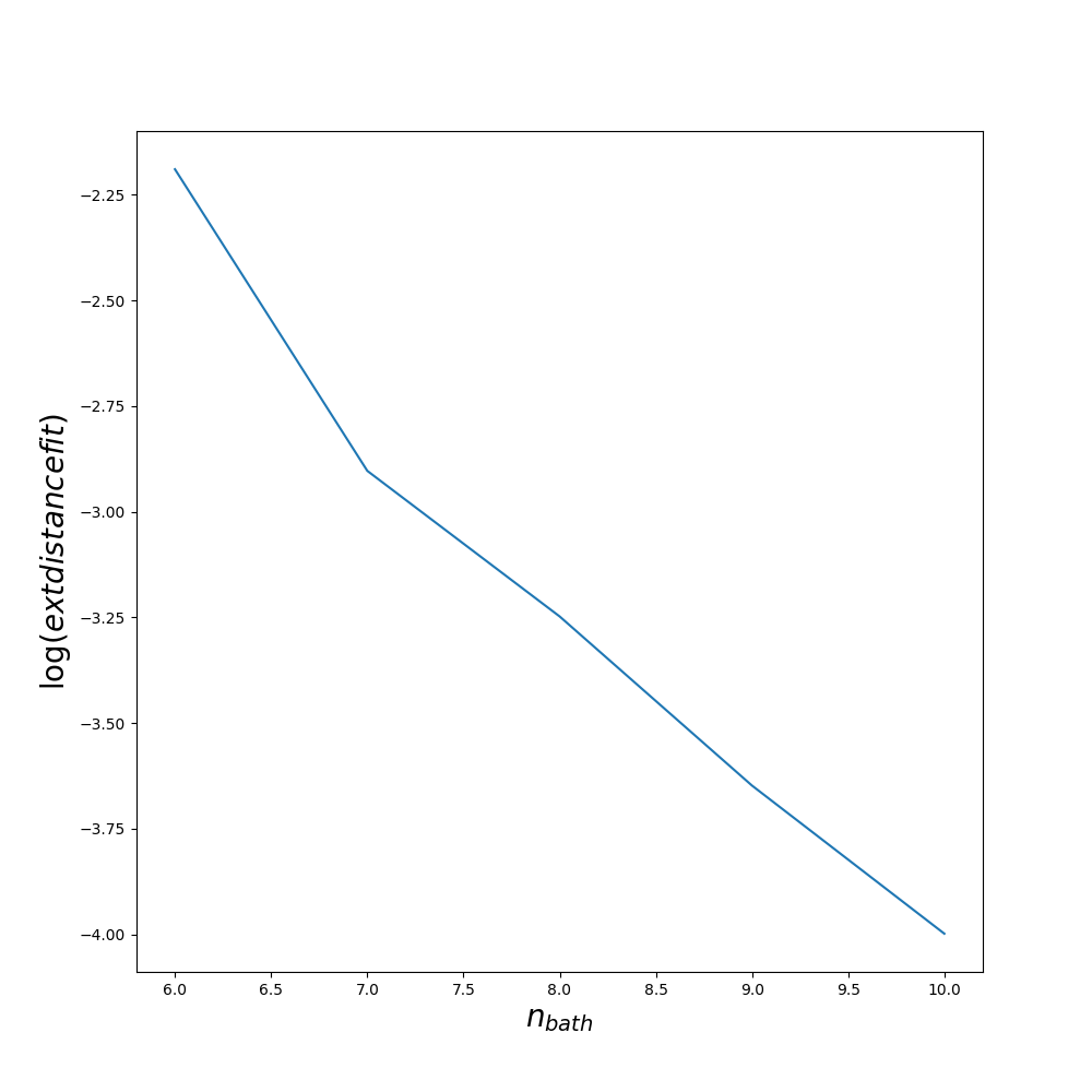
The quality of the fit is measured by the parameter called dist written in logfile-p1
  grep dist logfile-1
  [...]
  dist =    6.0058804019844005E-004        8000           0
In practice, above is a bad fit. below is good. This number depends of the number of points integrated in the fit which is controled by fit_nw in ED/ED.in.
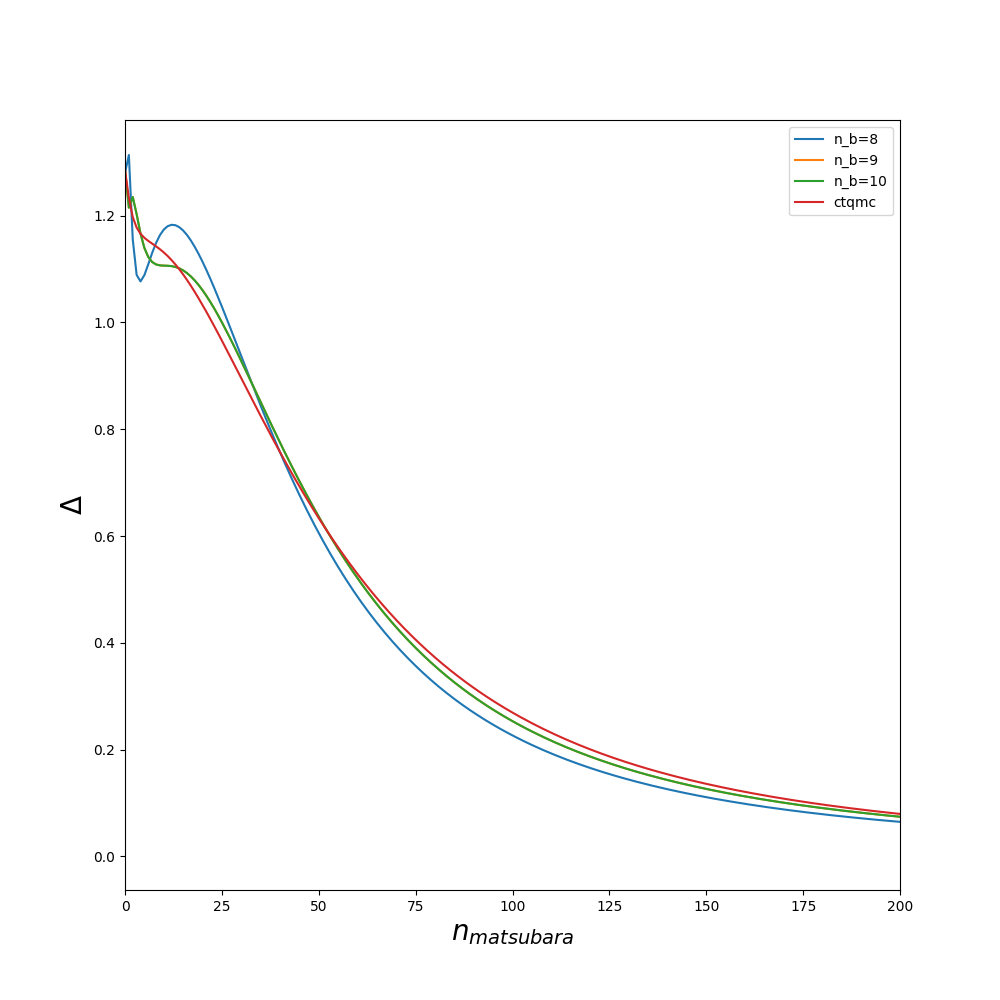
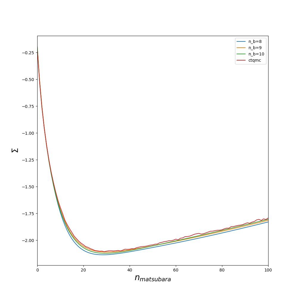
The quality of the fit could also be improved by increasing min_all_bath_param in ED/ED.in which controls the number of sites in the bath. It always a good idea before starting a full dmft loop to try several values of min_all_bath_parma and see how the result improved. An example is given on figures :
Lanczos
The Lanczos diagonalization is a great methods but should be use with caution. It is always good to play a bit with the parameter to be sure that the result is valid.
First try with normal lanczos for a small number of baths and compare with full_ed methods
Then increase the number of baths and look for ‘E0 =’ in the logfile-p1. It shows the energies for the different block. First you want to make sure that the code take into account some excited state. If not, you should increase Neigen to make it equal to 2 and increase dEmax0 which controles the maximum difference between ground state and excited state.
- If in some blocks, E1 exactly equal E0 then you are in trouble and should use Block_size=-1.
- If there is no excited state (i.e no E1), you should increase dEmax0
- If the result does not change, keep the parameter, the result is stabilized.
- If the result changes, increase Neigen by 1 and repeat the procedure.
Sometime, dEmax0 is to big with Block_size=-1 and result is bad. It is difficult to see it without a benchmark. Having a ctqmc benchmark is usefull in this case (It could be benchmarking without interband hopping for instance to avoid the sign problem). I would recommand to avoid using Block_size=-1.
DMFT LOOP
“lmed ybco –init” reads at each iteration the params file but does not overwrite ED/ED.in. It means that if someone configure ED/ED.in, for the first iteration, lmed –init will just modify and .
#Susceptibility
The susceptibility works only on mode FULL_ED, So . The computational cost grows as .
Go to imp_0
First modify ED/ED.in (at the end of the file), to be on the mode FULL_ED and
which_lanczos=FULL_ED
min_all_bath_param=6
Then run ed_solver and check if the self energy is not to far due to the small number of site.
If it is ok, create a file called mesh
nomb1
nomb2
nomf
roaming
- nomb1: integer, first bosonic frequency to compute (usually nomb1=1 which correspond to
- nomb2: integer, last bosonic frequency to compute
- nomf: number of fermionic frequency
- roaming: (.true./.false.) if true, center the fermionic grid to preserve the symmetry . Necessary for large bosonic frequency. If it is true, the fermionic grid must be shifted accordingly for $\chi_0$. It can be done by seting the token NOMB in ctrl to a negative number.
Run again ed_solver to generate the file c_transition
dmft_solver FLAG_DUMP_INFO_FOR_GAMMA_VERTEX=.true. Nitergreenmax=1 Neigen=20000 dEmax0=1000.0
The important number is demax0 since Neigen is set to a very large number. The code will include eigenstate up to an . if , in this case, , which is probably ok. The convergence of the result w.r.t this number should be checked. If it is too small, the tail of the vertex will not converge. The computational cost of the calculation grows as . As a remark, depends of the number of bath site.
Then, run vertex_ed. It can be run with openmpi/mpi. This part can be very demanding and, in general, need large cluster.
ulimit -s unlimited
export OMP_STACKSIZE=1g
env OMP_NUM_THREADS=32 mpirun -np 100 ed_vertex
return to the main directory
the ctrl file needs to be modified to have the bosinic/fermionic grid
DMFT NLOHI=2,10 BETA=50 NOMEGA=999 NOMF=10 NOMB=-3
The roaming mode for the fermionic grid is enabled.
Finally, run
lmed nio -rv
mpirun -np 30 lmfdmft --ldadc~fn=dc  --job=1 ctrl.nio
mpirun -np 30 lmfdmft --ldadc~fn=dc  --job=1 --chiloc ctrl.nio
mpirun -np 30 susceptibility
The vertex can be dumped in chiSQ.h5 with
mpirun -np 30 susceptibility --store_vertex