In this tutorial, we will apply dynamical mean field theory (DMFT) on Sr2RuO4 on a QSGW stating point that you can find here
Impurity solver
Questaal package does not supply an impurity solver. There are several choices of solver on the market, in this tutorial, the CTQMC solver from the TRIQS package is used (see TRIQS package and its hybridization-expansion solver solver) TRIQS is already installed on the machine used for this workshop.
Prepare Input folder and files
Go the the dmft folder present in your work directory
cd ~/work/
cp -r /home/vol06/tmp16/work/dmft_sr2ruo4 .
cd dmft_sr2ruo4
If you list your directory now, you should have :
atm.sr2ruo4 basp.sr2ruo4 ctrl.sr2ruo4 rst.sr2ruo4 sigm.sr2ruo4 site.sr2ruo4
Definition of the correlated subspace
At the end of ctrl file add the following :
DMFT    BETA=30 NOMEGA=999 NLOHI=16,42
        BLOCK:
        SITES=3 L= 2
        SIDXD= 1 2 0 2 0
Remark: Make sure you have the right indentation between the token DMFT and BLOCK.
Projection window
The first tokens have means :
- BETA=30 : The DMFT loop is done at inverse temperature (ev^-1) 30.
- NOMEGA : Number of Matsubara frequencies for the impurity self energy.
NLOHI=16.42 The projector are constructed with the bands from 16 to 42.
In principle, the window is infinite and all the bands should be included. In practice, for numerical reasons, we choose a large finite windows around the d-state.plot the partial dos on Ru atom (see tutorial here
mpirun -np 24 lmf sr2ruo4 -vnkabc=8 --quit=rho --pdos~mode=2~sites=3~lcut=2
lmdos sr2ruo4 -vnkabc=8 --quit=rho --pdos~mode=2~sites=3~lcut=2 --dos:npts=1001:window=-1,1
echo 1.4 5 -20 20 | pldos -fplot~sh~long~open~tmy=.25~dmin=0.40~xl=E -esclxy=13.6 -ef=0 -lst="5;6;7;8;9" dos.sr2ruo4
which prints a file fplot.ps that you can open with evince :
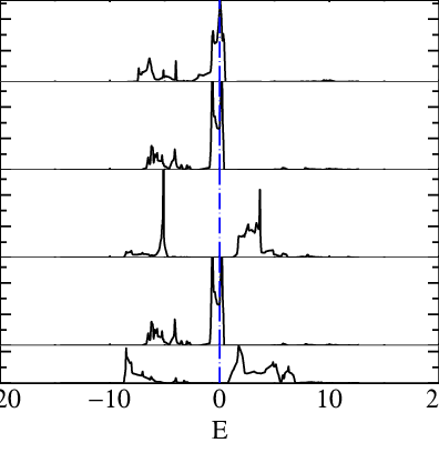
Panel 1,2,4 are t2g bands and 3,5 are eg.
In this tutorial, we will include the t2g bands so we want at least a windows at least of around -8 ev (0.58 Ry) to 8 eV the following command :
mpirun -np 24 lmf ctrl.sr2ruo4 --minmax --quit=rhoprints an array with the lower and higher energies (in Ry) of each bands over the Brillouin zone.
   1  -3.1933 -3.1923  |   65   1.8788  2.0501  |  129   4.7309  4.9919
 2  -3.1932 -3.1922  |   66   1.9419  2.0890  |  130   4.8393  5.0922
 3  -3.1661 -3.1658  |   67   1.9731  2.1264  |  131   4.9053  5.1016
 4  -2.6274 -2.6215  |   68   2.0040  2.1605  |  132   4.9440  5.1585
 5  -2.6228 -2.6196  |   69   2.0555  2.2153  |  133   4.9919  5.1952
 6  -1.5204 -1.4365  |   70   2.0900  2.3107  |  134   5.0455  5.2968
 7  -1.4430 -1.4355  |   71   2.1252  2.3360  |  135   5.0776  5.3219
 8  -1.4108 -1.3802  |   72   2.1726  2.3635  |  136   5.1263  5.3914
 9  -1.3998 -1.3629  |   73   2.1764  2.4229  |  137   5.1329  5.4252
10  -1.3041 -1.2684  |   74   2.2579  2.4491  |  138   5.1656  5.4392
11  -1.2971 -1.2629  |   75   2.2928  2.5067  |  139   5.1886  5.4739
12  -1.2803 -1.2585  |   76   2.3301  2.5856  |  140   5.2448  5.5131
13  -1.2747 -1.2463  |   77   2.3612  2.6184  |  141   5.3528  5.5326
14  -1.2558 -1.2075  |   78   2.4576  2.6479  |  142   5.3625  5.5800
15  -1.2405 -1.2064  |   79   2.5070  2.6812  |  143   5.4614  5.6184
16  -0.5752 -0.3531  |   80   2.5863  2.7187  |  144   5.4849  5.6598
17  -0.5550 -0.3531  |   81   2.6036  2.7533  |  145   5.5521  5.7134
18  -0.4820 -0.3084  |   82   2.6140  2.7589  |  146   5.6148  5.8006
19  -0.3974 -0.2972  |   83   2.6419  2.7795  |  147   5.6710  5.8289
20  -0.3743 -0.2419  |   84   2.6690  2.8733  |  148   5.6927  5.8528
21  -0.3121 -0.2289  |   85   2.6750  2.8797  |  149   5.7224  5.9200
22  -0.2710 -0.1819  |   86   2.6853  2.9270  |  150   5.7843  5.9534
23  -0.2607 -0.1755  |   87   2.7066  2.9472  |  151   5.8318  6.0230
24  -0.2219 -0.1618  |   88   2.7538  2.9835  |  152   5.8502  6.0298
25  -0.2137 -0.1341  |   89   2.8097  3.0046  |  153   5.8637  6.0883
26  -0.1670 -0.1281  |   90   2.8142  3.0375  |  154   5.9125  6.1391
27  -0.1506 -0.1118  |   91   2.8543  3.0865  |  155   5.9572  6.1855
28  -0.1404  0.0948  |   92   2.8951  3.1151  |  156   6.0318  6.2192
29   0.0028  0.0966  |   93   2.9317  3.1592  |  157   6.0892  6.2885
30   0.0028  0.1064  |   94   3.0004  3.1984  |  158   6.1307  6.3278
31   0.1241  0.3452  |   95   3.0451  3.2332  |  159   6.1794  6.4674
32   0.2157  0.4878  |   96   3.1038  3.2800  |  160   6.2245  6.4991
33   0.3272  0.5175  |   97   3.1583  3.3322  |  161   6.2727  6.5368
34   0.3602  0.5757  |   98   3.1991  3.4632  |  162   6.2787  6.6025
35   0.4733  0.6402  |   99   3.2188  3.5471  |  163   6.3411  6.6706
36   0.5218  0.6815  |  100   3.2625  3.5473  |  164   6.4144  6.6974
37   0.5741  0.7266  |  101   3.2988  3.5809  |  165   6.4714  6.7229
38   0.6189  0.7492  |  102   3.3689  3.6773  |  166   6.5543  6.8148
39   0.6359  0.8077  |  103   3.4046  3.6939  |  167   6.6090  6.8661
40   0.6657  0.8407  |  104   3.4186  3.7622  |  168   6.6523  6.9259
41   0.7294  0.8681  |  105   3.4595  3.8401  |  169   6.6834  7.0081
42   0.7714  0.8902  |  106   3.5179  3.8615  |  170   6.7564  7.0302
43   0.7813  0.9216  |  107   3.5787  3.8777  |  171   6.8423  7.1140
44   0.8269  0.9935  |  108   3.6858  3.9177  |  172   6.9238  7.1336
45   0.9261  1.0750  |  109   3.7300  3.9602  |  173   6.9394  7.2033
46   0.9507  1.1757  |  110   3.7610  3.9689  |  174   6.9742  7.2077
47   1.0236  1.2357  |  111   3.8346  4.0433  |  175   6.9983  7.2563
48   1.0793  1.2666  |  112   3.8837  4.0809  |  176   7.0628  7.3006
49   1.1336  1.2692  |  113   3.9219  4.0896  |  177   7.1292  7.4603
50   1.1579  1.4529  |  114   3.9735  4.1142  |  178   7.2345  7.5412
51   1.1790  1.4529  |  115   4.0064  4.1494  |  179   7.2853  7.5598
52   1.2092  1.4693  |  116   4.0548  4.2091  |  180   7.3522  7.7069
53   1.2931  1.5363  |  117   4.1113  4.2737  |  181   7.4270  7.7541
54   1.3212  1.6060  |  118   4.1363  4.3192  |  182   7.4274  7.9015
55   1.3494  1.6485  |  119   4.1976  4.3858  |  183   7.6705  7.9530
56   1.4468  1.6525  |  120   4.2307  4.4231  |  184   7.8429  8.3109
57   1.4956  1.7020  |  121   4.2748  4.5355  |  185   7.9566  8.5638
58   1.5960  1.7095  |  122   4.3247  4.5716  |  186   8.1509  9.1719
59   1.6300  1.7828  |  123   4.4494  4.6198  |  187   8.3788  9.5613
60   1.7048  1.8179  |  124   4.5232  4.6966  |  188   8.3801  9.5618
61   1.7308  1.9218  |  125   4.5748  4.7578  |  189   8.5248  9.7693
62   1.7599  1.9445  |  126   4.6161  4.7945  |  190   9.8480 10.0328
63   1.8104  1.9558  |  127   4.6564  4.8879  |  191   9.9069 10.8707
64   1.8320  1.9920  |  128   4.6564  4.9164  |
For this tutorial NLOHI=16,42
Definition of the impurity
In our example, the correlated subspace is composed of Ru d-state. This information is given by :
        BLOCK:
        SITES=3 L= 2
        SIDXD= 1 2 0 2 0
The DMFT subspace can have several correlated atoms. each correlated atoms is defined with it index in the site file, the orbital caracters of the corraleted orbital (l=2 for d, l=3 for f).
- SITES : index of correlated site (Here Ru which is the atom 3 in site file
- L : orbital momentum of correlated subspace (L=2 for d)
- SIDXD indicates which m =[-l .. +l] are taken into account in the impurity self energy To included off-diagonal term, SIDXD has to be replaced SIDXM and a (2L+1)x(2L+1) matrix has to be supplied. Here we take into accout xy, yz, xz where yz and xz are equivalent. The order in given by Questaal’s ordering
# Autogenerated from init.sr2ruo4 using:
# /users/ms4/bin/blm --gw --express=1 --nk=12 --nkgw=6 --gmax=11.0 --nit=100 sr2ruo4
% const nit=100
% const met=5
% const so=0 nsp=so?2:1
% const lxcf=2 lxcf1=0 lxcf2=0
% const pwmode=0 pwemax=3
% const sig=12 gwemax=2.46 gcutb=3.1 gcutx=2.5
% const nkabc=12 nkgw=6 gmax=11 beta=.3

VERS  LM:7 FP:7 # ASA:7
IO    SHOW=f HELP=f IACTIV=f VERBOS=35,35  OUTPUT=*
EXPRESS
  file=   site
  nit=    {nit}
  mix=    B2,b={beta},k=7
  conv=   1e-5
  convc=  3e-5
  nkabc=  {nkabc}
  metal=  {met}
  nspin=  {nsp}
  so=     {so}
  xcfun=  {lxcf},{lxcf1},{lxcf2}

#SYMGRP i r4z mx
HAM   GMAX={gmax}
      AUTOBAS[PNU=1 LOC=1 MTO=4 LMTO=5 GW=1 PFLOAT=2,1]
      PWMODE={pwmode} PWEMIN=0 PWEMAX={pwemax} OVEPS=0
      XCFUN={lxcf},{lxcf1},{lxcf2}
      FORCES={so==0} ELIND=-0.7 NSPIN={nsp} SO={so}
      RDSIG={sig} SIGP[EMAX={gwemax}]
ITER  MIX=B2,b={beta},k=7  NIT={nit}  CONVC=1e-5
BZ    METAL={met}  NKABC={nkabc}
GW    NKABC={nkgw} GCUTB={gcutb} GCUTX={gcutx} DELRE=.01 .1
      GSMEAR=0.003 PBTOL=3e-4,3e-4,1e-3
STRUC
      SHEAR=1 0 0 1.0
      NL=5  NBAS=7  NSPEC=3
      ALAT= 7.30111097
      PLAT= -0.5  0.5  1.6455593  0.5  -0.5  1.6455593  0.5  0.5  -1.6455593
SPEC
  ATOM=Sr       Z= 38  R= 2.985910  LMX=3 LMXA=4
  ATOM=Ru       Z= 44  R= 2.068587  LMX=3 LMXA=4 PZ=0,0,5.4
  ATOM=O        Z=  8  R= 1.581969  LMX=3 LMXA=4
SITE
  ATOM=Sr         POS=  0.5000000   0.5000000  -0.4851109
  ATOM=Sr         POS= -0.5000000  -0.5000000   0.4851109
  ATOM=Ru         POS=  0.0000000   0.0000000   0.0000000
  ATOM=O          POS=  0.0000000   0.5000000   0.0000000
  ATOM=O          POS=  0.0000000   0.0000000   0.5348068
  ATOM=O          POS= -0.5000000   0.0000000   0.0000000
  ATOM=O          POS=  0.0000000   0.0000000  -0.5348068
DMFT    NLOHI=16,42 BETA=30 NOMEGA=999
        BLOCK:
        SITES=3 L= 2
        SIDXD= 1 2 0 2 0
Double Counting
We will use a static double counting given by the fully localized limit (FLL), with U = 4.5 eV, J = 1 eV, n = 4
Edc = U(n-1/2)-J(n-1)/2 = 14.25 eV
echo "14.25 14.25" > dc.sr2ruo4 # there is one value for each independant active orbital
Solver parameters
The CTQMC solver is a Monte Carlo solver. The parameters needed by the solver are given in para_triqs.txt. In this tutorial, we just need one params file. An example is given below :
U 4.5
J 1
n_warmup_cycles 100000
n_cycles 300000
length_cycle 30
n_l 50
- U : Effective interation
- J : Hund coupling
- n_warmup_cycles : number of warmup steps.
- n_cycles : number of measures per core
- length_cycle : number of steps between two measures. If this number is too small, the data will be noisy due to correlated sampling. If this number is too large, the calculation will be longer uselessly.
- n_l : number of Legendre coefficients (see [3])
Put the parameters above in a file called para_triqs.txt
Note: The total number of measures is n_cycles*number_of_cores. So increasing the number of core will increase the quality of the result.
First iteration
In general, it is adviced to perform the first iteration and check the quality of the result in order to be sure than the number set in para_triqs.txt are ok.
Create a new folder for the first iteration
mkdir it1
cp -f * it1/.
cd it1/
In it1, run lmfdmft to create a self energy file sig.inp
lmfdmft sr2ruo4 --ldadc~fn=dc --job=1
this command creates a file sig.inp
there is NOMEGA lines Then the structure of the collun is
w Re(S_1) Im(S_1) ... Re(S_i) Im(S_i)
where i is the index given in the token SIDXD or SIDXM
Once the file sig.inp is created, run again
mpirun -np 24 lmfdmft sr2ruo4 --ldadc~fn=dc --job=1
It will create the file solver_input.h5 which is a hdf5 file format.
Let try to run the ctqmc solver now.
mpirun -np 24 lmtriqs sr2ruo4
The calculation takes about 10 minutes. In the plot show below, we run the calculation on 24 cores.
The first thing to check is that the number of Legendre coefficient for the Green function is correct. it has to be high enough so the coefficient goes to zeros. If it is too high, the high coefficient just contained Monte Carlo noise which pollutes the final result.
nb_of_legendre_coef Re(G_l_1_up) ... Re(G_l_i_up) .... Re(G_l_1_down) ...
A simple python script to plot it could be :
import numpy as np
import matplotlib.pyplot as plt
import sys
Gl = np.loadtxt(sys.argv[1]).T
wl = Gl[0]
Gl = Gl[1:]
#plot just G_l_up
for i in range(Gl.shape[0]) :
    plt.plot(wl,Gl[i])
plt.xlabel('n_l')
plt.ylabel('Gl')
plt.savefig('gl.png')
plt.show()
put this script in a file plot_gl.py and run
python plot_gl.py path_to/gl.inp
You should obtain :
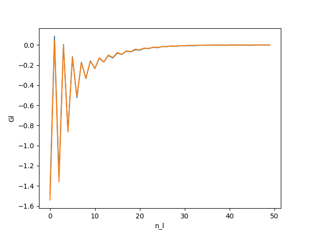 All the coefficients go to 0.
Then, the Green function on the Matsubara axis is deduced from G_l and the self energy is obtained from the Dyson equation.
The self energy is contained in the file sig.inp
A simple python script to plot sig.inp could be :
import numpy as np
import matplotlib.pyplot as plt
import sys
S = np.loadtxt(sys.argv[1]).T
w = S[0]
Sig = S[1::2] + 1j* S[2::2]
#plot just Sig_up
plt.figure(figsize=(8,8))
for i in range(Sig.shape[0]) :
    plt.plot(w,Sig[i].imag,label=i+1)
plt.xlabel(r'$\Omega_n$', fontsize = 20)
plt.ylabel(r'$\Sigma$', fontsize = 20)
plt.xlim(0,200)
plt.legend()
plt.savefig('sig_sr2ruo4.png')
plt.show()
put this script in a file plot_giw.py and run
python plot_giw.py path_to/sig.inp
You should obtain :
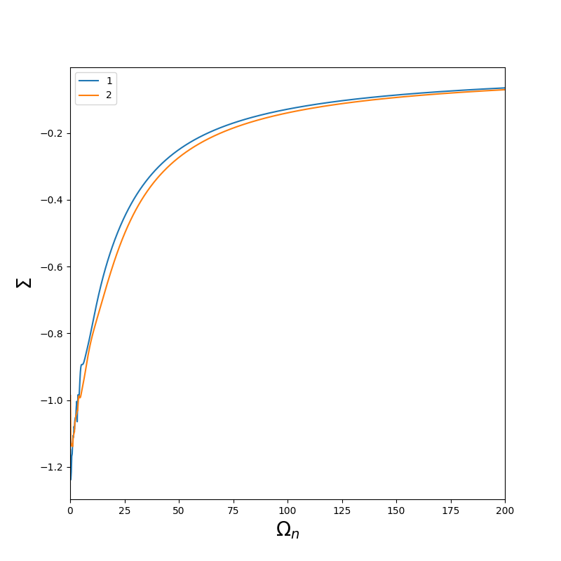
The self energy of the second orbital is noiser than the first one because the second one is the average of yz and xz.
To complete the dmft loop, we need to run again lmfdmft to get a updated hybridisation function and impurity energy level and then run again the impurity solver to get a new self energy. It has to be repeated until convergence.
DMFT loop
To perform the DMFT loop, we proposed a bash script which could be adapted for your machine. It’s assumed that you have set correctly the ctrl file and the params file
#!/bin/bash -l
set -xe


x=sr2ruo4
mxit=20 # nb of iteration
np_lmfdmft=24 # nb of cores available for lmfdmft
np_ctqmc=24 # nb of cores available for lmfdmft


if [ ! -e it1 ]; then
    mkdir -p it1
    cp -f * it1/.
fi

for i in `seq $mxit`;
do
    [ ! -e "it$((i-1))" ] || [ ! -e "it${i}"  ] || continue # if some iterations have already be done ...
    [ ! -e "it$((i-1))" ] || [ -e "it${i}"  ] || cp -av "it$((i-1))" "it${i}"
    pushd "it${i}"

    mpirun -n $np_ctqmc  lmfdmft --ldadc~fn=dc -job=1 ctrl.$x
    rm -f evec* proj*
    mpirun -np $np_ctqmc lmtriqs $x
    popd
done
It is adviced to check the convergence by plotting the difference sig.inp in each itX folder. It is also adviced to perform the average over the last iteration.
You can find a converged result in
extra/sig_converge.inp
For the rest of the tutorial replace your sig.inp by the converge one:
cp extra/sig_converge.inp sig.inp
This has been converged using 30 iterations and average on the 10 last interation (with n_cycles=1000000) on a 24 cores machine.
Analyse of the result
Analytic continuation
In this tutorial we use lmfdmft’s built in Pade extrapolator to carry out the analytic continuation.
Note: analytic continuation is a tricky business. Pade works reliably only when the polynomial order is not too large, which means in can operate reliably only over a small energy window. Also the self-energy should be reasonably smooth.
lmfdmft sr2ruo4 --rs=1,0 --ldadc~fn=dc -job=1 --pade~nw=121~window=-6/13.606,6/13.606~icut=30,75
it creates a file sig2.sr2ruo4 containing the self energy in the real axis which has the same format than sig.inp.
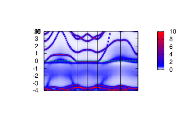
Spectral function
In this section, the spectral function
To do so, execute the following command.
 cp extra/syml.sr2ruo4 . # copy the symetry lines.
 mpirun -np 24 lmfdmft sr2ruo4  --rs=1,0 --ldadc~fn=dc -job=1 --gprt~band,fn=syml~rdsigr=sig2~mode=19
 lmfgws sr2ruo4 '--sfuned~units eV~readsek@useef@irrmesh@minmax~eps 0.02~se band@fn=syml nw=2 isp=1 range=-4,4'
 plbnds -sp~atop=10~window=-4,4 spq2.sr2ruo4
 gnuplot gnu.plt
Spectrum DOS
QSGW noninteracting DOS
Making the QSGW noninteracting DOS using lmf in the usual manner, using the --dos switch
lmf sr2ruo4 -vnkabc=12 --dos@npts=721@ef0@rdm@window=-6/13.606,6/13.606 --quit=dos
Note: you could speed up the calculation by using mpi.
It creates file dos.sr2ruo4. --quit=dos tells lmf to stop after the DOS has been written, and the modifies to --dos have the following meanings:
- npts=721 specifies number of energy points (the spacing between points is the same as for the spectrum dos)
- window=−6/13.606,6/13.606 energy window for DOS, in Ry. It is 3/2 wider than that generated for the spectrum DOS
- ef0 Energy window to be defined relative to Fermi level
- rdm Write DOS in standard Questaal format for 2D arrays.
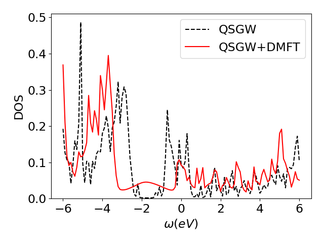
DMFT interaction DOS
lmfdmft sr2ruo4 -vnkabc=8 --ldadc~fn=dc --job=1 --gprt~rdsigr=sig2~mode=19
lmfgws sr2ruo4 -vnkgw=8 '--sfuned~units eV~readsek@useef@ib=1:27~eps 0.02~dos isp=1 range=-4,4 getev=12 nw=4~savesea~q'
Note: you can speed up the calculation by using mpi for lmfdmft but mpi does not work with lmfg
To compare the two DOS, you can use the fplot utility :
fplot -vef0=0.00037 sdos.sr2ruo4 -ab '(x1-ef0)*13.6' -ord x2/13.6 -lt 2,col=1,0,0 dos.sr2ruo4
The noninteracting DOS are written in Ry, on an absolute energy scale (i.e. not relative to the Fermi level).
-ab ‘(x1-ef0)*13.6’ shifts by ef0 and scales the abscissa from Ry to eV. -ord x2/13.6 scales the ordinate from Ry−1 to eV−1.
Spin susceptibility
The spin susceptibility is obtained from the local vertex :
The DMFT vertex is obtained from the local susceptibility :
impurity susceptibility
The local susceptibility is obtained from the two particle green function :
The two-particles Green function has 1 bosonic frequency, 2 fermionic frequencies and 2 orbital indicies (formally 4 but we do not take into account off-diagonal terms in this tutorial). This quantity is computed by the TRIQS cthyb solver.
The first step is to modify the line with DMFT token on the ctrl file by :
DMFT NLOHI=16,42 BETA=30 NOMEGA=999 NOMF=50 NOMB=1
- NOMF=50 : Number of fermionic frequencies to included in the local susceptibility
- NOMB=1 : Number of bosinic frequencies to included in the local susceptibility
The computation of the two particle Green function severaly slows the solver. In this case, it is good to increase length_cycle in the para_triqs file and reduce n_cycles.
For the purpose of this tutorial, the local susceptibility has already be computed on a 240 cores machine with the following para_triqs.txt file :
U 4.5
J 1.0
n_warmup_cycles 100000
n_cycles 100000
length_cycle 500
n_l 50
and run
mpirun -np 24 lmfdmft sr2ruo4  --ldadc~fn=dc --job=1 # makes sure that solver_input.h5 are update
mpirun -np 24 lmtriqs sr2ruo4 --vertex
it takes around 9 hours.
In your folder, do :
cp extra/chiloc_1_example.h5 chiloc_1.h5
The is computed by lmfdmft.
can be computed on the 1 Brillouin zone or in a given q mesh. This q mesh has be given as follow : the first term is the size of the k mesh (should be equal to nkabc in the ctrl file (this option works for nkabc(1)=nkabs(2)=nkabs(3)). then on each line, q is given by :
where Q_1, Q_2, Q_3 are the reciprocal lattice vector and
For instance, the following q list describes a q line along for to on 9x9x9 q-mesh.
9
0 0 0
0 0 1
0 0 2
0 0 3
0 0 4
0 0 5
0 0 6
0 0 7
0 0 8
put the q-list in a file called “qlist” and then run :
mpirun -np 24 lmfdmft sr2ruo4 -vnkabc=9 --ldadc~fn=dc --job=1 --chiloc --qlist
Remark: To make and the full BZ, just remove the –qlist flag.
Finally the Bethe Salpeter equation is done by running :
susceptibility
it stores the susceptibility in a h5 format and in a txt file called chi_spin.txt :
#iq iom real(chi)    imag(chi)
 0  0  13.3551597356 4.90070946787e-13
 1  0  14.8699746786 2.31342722756e-12
 2  0  17.6681324135 8.23262199153e-12
 3  0  12.0345500361 8.8882197898e-12
 4  0  7.24252562004 3.83866087065e-12
 5  0  7.24252562004 4.06060740588e-12
 6  0  12.0345500361 8.91117180046e-12
 7  0  17.6681324135 8.94648059339e-12
 8  0  14.8699746786 2.30697313105e-12
You can then plot it with your favorite program.
References
[1] K. Haule, C.H. Yee, and K. Kim. Dynamical mean field theory within the full-potential methods: Electronic structure of ceirin5, cecoin5, and cerhin5. Phys. Rev. B, 81:195107, 2010.
[2] Paolo Pisanti. A novel QSGW+DMFT method for the study of strongly correlated materials. PhD thesis, King’s College London, 2016.
[3] Lewin Boehnke et al. “Orthogonal polynomial representation of imaginary-time Green’s functions”. Physical Review B 84.7 (2011).