Dielectric functions and exciton visualisations
Introduction
This tutorial shows how to calculate dielectric functions with QSGW and ladder diagram corrected QSGW (a.k.a. QSGŴ a.k.a QSGW~).
A few launcher definitions which may come handy
m1="env OMP_NUM_THREADS=32 MKL_NUM_THREADS=32 mpirun -n 1 -ppn 1"
mn="env OMP_NUM_THREADS=1 MKL_NUM_THREADS=1 mpirun -n 32 -ppn 32"
md="env OMP_NUM_THREADS=2 MKL_NUM_THREADS=2 mpirun -n 16 -ppn 16"

s=/mnt/ceph-training/course_materials/LiF/4s/i
Basic input generation has been shown multiple times already so let’s move on and just copy the necessary files.
Dielectric functions
A quick DFT/LDA calculation
rsync -av $s/ lda/

pushd lda

$m1 lmfa --v8 ctrl.lm | tee llmfa
$mn lmf --v8 ctrl.lm | tee llmf
See if the bandstructure looks reasonable, first make sure the Fermi level is current
$mn lmf --v8 --quit=band ctrl.lm | tee lef
Now generate bands data. Weights grouped by element is optinal but nice to have.
$mn lmf --v8 --band~fn=syml~scol:atom=Li~scol2:atom=F ctrl.lm | tee lbnds
Plot bands, colouring the groups with semi-transparent red and blue respectively, also skip the empty space between 0.5 and 8 eV because LiF is a very wide gap insulator.
band-plot syml.lm bnds.lm:c=#00000080,#80000080,#00008080 -e -5,0.5,8,40 -o bands.pdf

popd
QSGW
Get a QSGW self-energy
rsync -av $s/ lda/rst.lm qsgw/

pushd qsgw

lmgw.sh --mpirun-1="$m1" --mpirun-n="$mn" --cmd-gd="$md" --lm-flags="--v8" --no-scrho ctrl.lm | tee llmgwsc
Band plotting song and dance
$mn lmf --v8 --quit=band ctrl.lm | tee lef
$mn lmf --v8 --band~fn=syml~scol:atom=Li~scol2:atom=F ctrl.lm | tee lbnds
band-plot syml.lm bnds.lm:c=#00000080,#80000080,#00008080 -e -5,0.5,8,40 -o bands-qsgw.pdf
Adjust settings in section optics and calculate the dielectric function for a specified q point (near Γ in this case)
lmgw.sh --epsq --mpirun-1="$m1" --mpirun-n="$mn" --cmd-gd="$md" --lm-flags="--v8" --no-scrho ctrl.lm | tee llmgw-epsq
mv eps.h5 epsq-qsgw.h5
Macroscopic ε from single shot BSE on top of QSGW, the band plot can guide active space selection for the BSE solver, here we stick with a rough v4c4 configuration. A quality calculation will need to converge the numbers of states and q-mesh in addition to the lower level convergence parameters.
lmgw.sh --bse --mpirun-1="$m1" --mpirun-n="$mn" --cmd-gd="$md" --lm-flags="--v8" --no-scrho ctrl.lm | tee llmgw-eps-bse
mv eps-plot.txt eps-qsgw-bse.txt

popd
QSGŴ
Get a QSGW~ self-energy accounting for the additional screening to W from excitonic effects. Starting from QSGW Σ, thought it possible to start from LDA too, the final result is the same withing tolerance given the LDA state is nonmetallic (which is case with LiF).
rsync -av $s/ qsgw/rst.lm qsgw/sigm.lm qsgw/sig.h5 bsw/

pushd bsw

lmgw.sh --bsw --mpirun-1="$m1" --mpirun-n="$mn" --cmd-gd="$md" --lm-flags="--v8" --no-scrho ctrl.lm | tee llmgww
Band plotting again
$mn lmf --v8 --quit=band ctrl.lm | tee lef
$mn lmf --v8 --band~fn=syml~scol:atom=Li~scol2:atom=F ctrl.lm | tee lbnds
band-plot syml.lm bnds.lm:c=#00000080,#80000080,#00008080 -e -5,0.5,8,40 -o bands-qsgww.pdf
The macroscopic ε from QSGŴ
lmgw.sh --bse --mpirun-1="$m1" --mpirun-n="$mn" --cmd-gd="$md" --lm-flags="--v8" --no-scrho ctrl.lm | tee llmgww-eps-bse
mv eps-plot.txt eps-qsgww-bse.txt
Plot all the ε with your tool of choice and compare, the data is fairly simple, or find an example matplot script:
$s/../eps-plot.py
The dielectric function can be fed into various external tools which can show how the material will look/what colour it will have under given illumination.
Exciton postprocessing
The stdout saved in file “lbse” has the list of the bound excitons found, together with some basic info to guide further steps, here is an excerpt:
spin 1 evals in [-3.7181, -.9006] Ry
writing restart data to file w2q0e.h5 ... done

Macroscopic dielectric function on uniform frequency mesh in window (0,2) spacing 1e-3  broadening (-0.083,0.107)


344 evals in range: [.000,1.658], grouped by degeneracy tol .1000E-02ry
isp  hidx  group    ev, ry            ev, ev         oscillator strengths along qvecs
 0   1023     0    0.90058622        12.253100        5.527       0.1699       0.1441
 0   1022     0    0.90058693        12.253109       0.2581       0.7705        4.813
 0   1021     0    0.90058705        12.253111       0.5581E-01    4.901       0.8845
 0   1020     1    0.99760367        13.573089        3.397       0.2102       0.2090
 0   1019     1    0.99760423        13.573097       0.3127       0.1869        3.316
 0   1018     1    0.99760435        13.573099       0.1065        3.419       0.2907
 0   1017     2     1.0377768        14.119672       0.1440E-20   0.5671E-20   0.2907E-20
 0   1016     2     1.0377769        14.119674       0.4442E-21   0.3193E-20   0.3319E-21
 0   1015     2     1.0377769        14.119675       0.6906E-20   0.2075E-20   0.2699E-21
 0   1014     3     1.0420110        14.177282       0.3711E-21   0.5395E-20   0.2938E-20
 0   1013     3     1.0420111        14.177283       0.1026E-22   0.5096E-21   0.3853E-20
 0   1012     4     1.0432273        14.193830       0.1237E-05   0.2525E-06   0.4518E-06
 0   1011     4     1.0432274        14.193832       0.1013E-06   0.6227E-06   0.1268E-05
 0   1010     4     1.0432276        14.193835       0.6639E-06   0.1119E-05   0.2823E-06
 0   1009     5     1.0471367        14.247020       0.1099E-09   0.8179E-10   0.2440E-09
 0   1008     5     1.0471368        14.247022       0.3635E-09   0.9916E-14   0.6990E-09
 0   1007     6     1.0582795        14.398626       0.2995E-20   0.2000E-20   0.5606E-23
 0   1006     6     1.0582797        14.398629       0.3137E-20   0.2159E-20   0.2467E-20
 0   1005     6     1.0582799        14.398632       0.4642E-21   0.9365E-22   0.5173E-22
 0   1004     7     1.0863261        14.780220       0.2404       0.2559       0.2128
 0   1003     7     1.0863263        14.780223       0.6871E-02   0.2697       0.4324
 0   1002     7     1.0863265        14.780225       0.4618       0.1834       0.6380E-01
 0   1001     8     1.0891523        14.818671       0.3175E-06   0.7265E-07   0.8461E-07
 0   1000     8     1.0891524        14.818674       0.1676E-10   0.1935E-06   0.2782E-06
 0    999     8     1.0891526        14.818675       0.2095E-06   0.2281E-06   0.1750E-06
 0    998     8     1.0897236        14.826444       0.7004E-09   0.1806E-09   0.1204E-08
 0    997     8     1.0897237        14.826446       0.6221E-11   0.3758E-09   0.4860E-09
The lowest exciton is ~12.25ev (group 0) and it is not dark as attested by the oscillator strengths in the different directions. We can try to quantify the level to which the active states participate in a particular exciton by integrating the 2 particle weights for a chosen energy range and decorate a band plot with them.
Preserve the printed bse command line for postprocessing steps, wich a small modidifaction: use just 1 process because the data from the previous step can be reused, the computational load is then minimal
bsc="$m1 bse --optdfl=optdatac.h5 --v8 ctrl.lm"
Band weights
Let’s start with the weights for energy window 12-13eV and record the output to a file named exbw-12-13ev.h5:
$bsc --wexbw~ewin=12,13eV~fn=exbw-12-13ev.h5
Now overlay it on the band picture, skip the colour weights for clarity now, though they can be useful to visually evaluate orbital projections, we’ll have a more formal estimation in the next step…
band-plot syml.lm bnds.lm -e -5,0.5,8,40 --exbw exbw-12-13ev.h5 -o bands-exbw-12-13.pdf
Note the colour is at present completely meaningless and can be set to single one with –exbw-colour (this may change with the introduction of orbital weights)
There are two immediate observations in this case: * while the occupied states have similar contributions, only the lowest unoccupied band seems to participate in a meaningful way * the exciton is of Wannier type, localised in q, likely spread out in r (to be seen).
Orbital weights
We can see how (de)localised and exciton is in r/direct space by plotting Ψ(r_h, r_e) or its square. Since covering the full (r_h, r_e) space for a reasonably dense r-mesh would require quite a bit of storage we fix one of the particles and let the other cover a supercell of size nk because this is the limit of the periodicity of the constituent single particle wavefunctions.
Two popular examples are to fix the hole on the F atom or electron on Li, however it is not always this obvious and there sometimes can be very many choices available. To narrow it down to a set of physically significant choices we can project to orbitals (calculate orbital weights) for selected exciton:
$bsc --wexow~ewin=12,13eV~fn=exow-12-13ev.h5 | tee exow-12-13.log
The following are the interesting bits from the output file
isp: 0 ei: 1023 ev: .90058622ry (12.253100ev) oscillator strengths: 5.527 .1699 .1441
v\c
   0.7346   0.0004   0.0013   0.0001
   0.1945   0.0007   0.0009   0.0002
   0.0665   0.0005   0.0004   0.0000
   0.0000   0.0000   0.0000   0.0000
 site class onsite:
               Li        F
            0.0193   0.0479
 site class intersite:
 v\c           Li⁻       F⁻
      Li⁺   0.2101   0.0908
       F⁺   0.4890   0.1430

 isp: 0 ei: 1022 ev: .90058693ry (12.253109ev) oscillator strengths: .2581 .7705 4.813
v\c
   0.1900   0.0003   0.0013   0.0001
   0.6808   0.0007   0.0008   0.0002
   0.1249   0.0005   0.0004   0.0000
   0.0000   0.0000   0.0000   0.0000
 site class onsite:
               Li        F
            0.0192   0.0480
 site class intersite:
 v\c           Li⁻       F⁻
      Li⁺   0.2101   0.0908
       F⁺   0.4890   0.1429

 isp: 0 ei: 1021 ev: .90058705ry (12.253111ev) oscillator strengths: .5581E-01 4.901 .8845
v\c
   0.2411   0.0004   0.0013   0.0001
   0.2283   0.0007   0.0008   0.0002
   0.5263   0.0005   0.0004   0.0000
   0.0000   0.0000   0.0000   0.0000
 site class onsite:
               Li        F
            0.0191   0.0479
 site class intersite:
 v\c           Li⁻       F⁻
      Li⁺   0.2102   0.0908
       F⁺   0.4890   0.1429
averaged site distribution from selected excitons:
 site class onsite:
               Li        F
            0.0192   0.0479
 site class intersite:
 v\c           Li⁻       F⁻
      Li⁺   0.2101   0.0908
       F⁺   0.4890   0.1429
It is now clear the largest weight is indeed on the Li⁻F⁺ pair and this supports the intuitive choice.
We can plot the atom weights with the following command:
exow-plot -s Li:0 -s F:1 exow-12-13.log
The output files are exow-12-13.log.pdf and exow-12-13.log.png, -s defines the specie name with its associated indexes in the matrix above in case there are multiple of the same due to disabled symmetry. There are a few useful options available, try --help for a description.
3D projections of Ψ(e,h)
To plot the 3d probability density for F⁺ case fix the hole (r+) at cartesian coordinate [-0.5,0,0] (the F atom), units of alat (see ctrl file for its value), swapping the c suffix with p switches to units of plat, useful if your input is in the same units (using xpos instead of pos in ctrl file):
$bsc --wexpsi~ewin=12,13eV~r+=-0.5,0.0,0.0c~fn=xcfh-f-12-13ev.xsf | tee xcfh-f-12-13ev.log
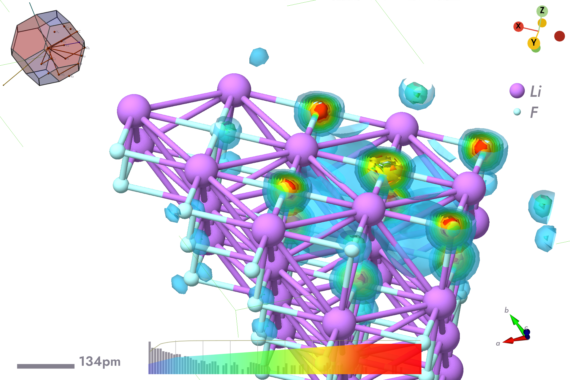
Electron probability density for hole fixed at centre of F atom.
For the Li⁻ case fix the electron (r-) at cartesian coortinate [0,0,0] (the Li atom):
$bsc --wexpsi~ewin=12,13eV~r-=0.0,0.0,0.0c~fn=xcfe-li-12-13ev.xsf | tee xcfe-li-12-13ev.log
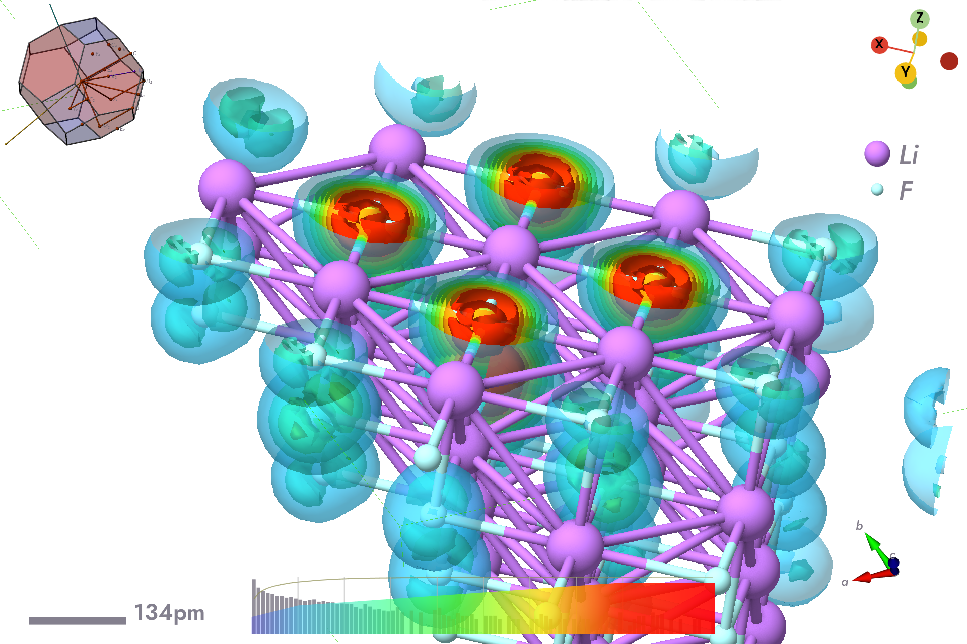
Hole probability density for electron fixed at centre of Li atom.
Increase gmax for better resolution 3d images, note the chosen position is shifted to nearest mesh point:
 integrating excitonic eigenstates over energy window [.8820, .9555] Ry
 ws                  1021
 wn                     3
 ngmx: 1892
 gmax: 10.00000000000000
 fmsh: 14 14 14
e⁻ at: .0000 .0000 .0000 alat
e⁻ at: .0000 .0000 .0000 plat, snap to ftmesh point: .0000 .0000 .0000 plat, deviation: .0000 .0000 .0000 alat
r range: [ -2.0000 -2.0000 -2.0000] to [ 2.0000 2.0000 2.0000]
 vs                     0 nv                     4
 cs                     4 nc                     4
 nr: 175616

 isp: 0 ei: 1023 ev: .90058622ry (12.253100ev) oscillator strengths: 5.527 .1699 .1441
v\c
   0.7346   0.0004   0.0013   0.0001
   0.1945   0.0007   0.0009   0.0002
   0.0665   0.0005   0.0004   0.0000
   0.0000   0.0000   0.0000   0.0000
 min: .2144299267731736E-19 max: .2325648338240825E-01 sum: 48.00384565657129

 isp: 0 ei: 1022 ev: .90058693ry (12.253109ev) oscillator strengths: .2581 .7705 4.813
v\c
   0.1900   0.0003   0.0013   0.0001
   0.6808   0.0007   0.0008   0.0002
   0.1249   0.0005   0.0004   0.0000
   0.0000   0.0000   0.0000   0.0000
 min: .3050129714594865E-20 max: .2296287535568177E-01 sum: 48.00354053522292

 isp: 0 ei: 1021 ev: .90058705ry (12.253111ev) oscillator strengths: .5581E-01 4.901 .8845
v\c
   0.2411   0.0004   0.0013   0.0001
   0.2283   0.0007   0.0008   0.0002
   0.5263   0.0005   0.0004   0.0000
   0.0000   0.0000   0.0000   0.0000
 min: .1111454789511420E-21 max: .2369849759362223E-01 sum: 48.00351253244630
The resulting volume data is saved in the specified xsf files which can be opened with various visualisation tools
What may yield better results is offsetting the fixed point slightly away from the atom centre to capture $\ell > 0$ components.
$bsc --wexpsi~ewin=12,13eV~r+=-0.5,0.0,0.1c~fn=xcfh-f-z0.1-12-13ev.h5 | tee xcfh-f-z0.1-12-13ev.log
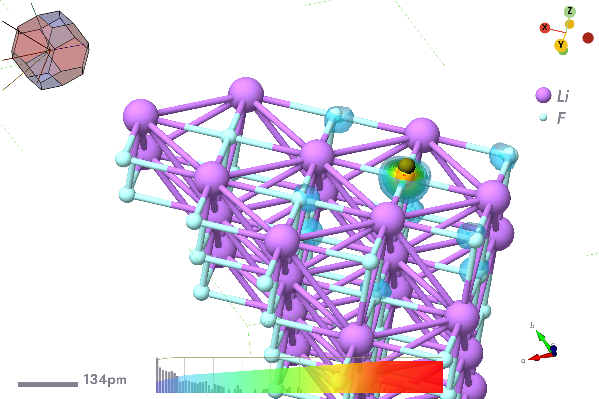
Electron probability density for hole fixed above F atom.
$bsc --wexpsi~ewin=12,13eV~r-=0.0,0.0,0.1c~fn=xcfe-li-z0.1-12-13ev.h5 | tee xcfe-li-z0.1-12-13ev.log
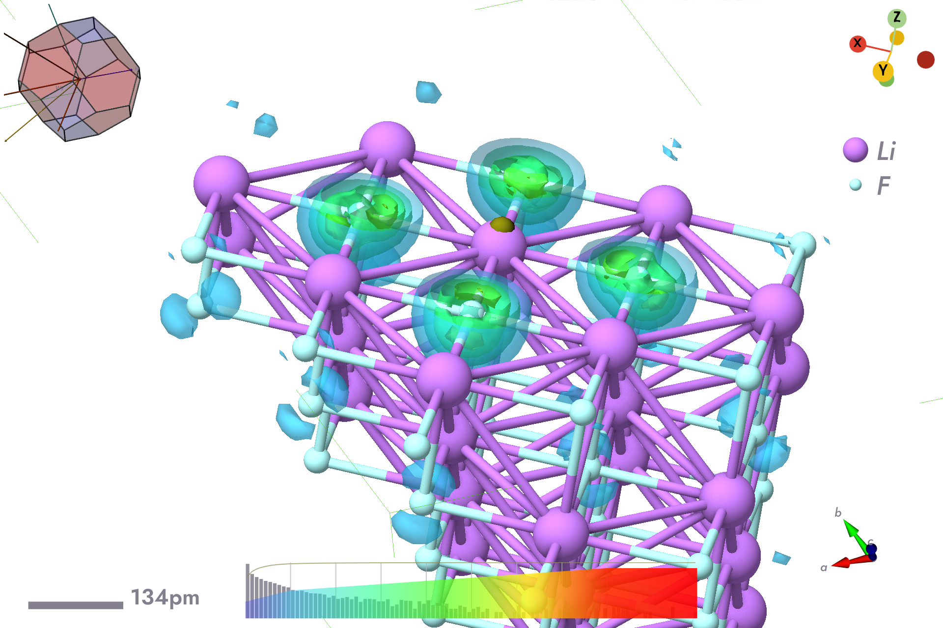
Hole probability density for electron fixed above Li atom.
Choosing an offset point is somewhat arbitrary, very different pictures can emerge depending on the direction of the point, also a point not on the ftmesh can yield complex projections. To spare some trouble and avoid ambiguity, one may wish to integrate all possible r point weighted by a chosen set of atomic orbitals, for example one associated with an atom. For the examples above this can be done with:
$bsc --wexrow~ewin=12,13eV~atom-=1~fn=exrow-li-e-12-13ev.h5 | tee exrow-li-e-12-13ev.log
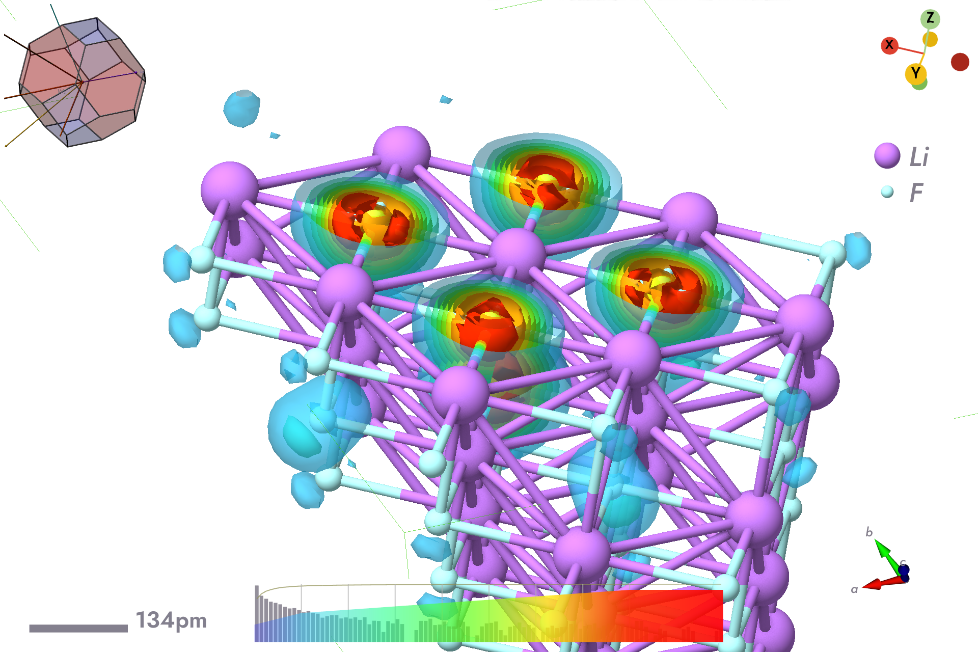
Electron probability density for hole weighted across whole space by F centered orbitals.
$bsc --wexrow~ewin=12,13eV~atom+=2~fn=exrow-f-h-12-13ev.h5 | tee exrow-f-h-12-13ev.log
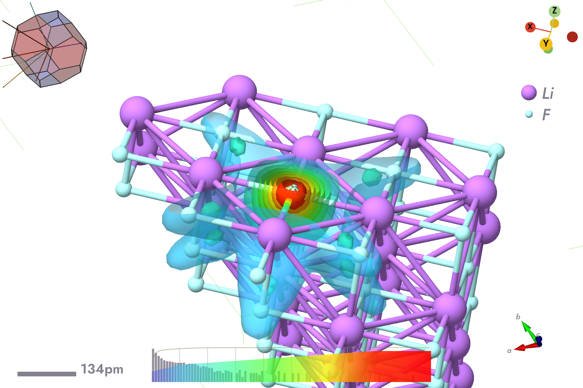
Hole probability density for electron weighted across whole space by Li centered orbitals.
Instead of ewin one can use eidx to supply a list of excitation eigenstates, add ~orth=1 to project on orthogonalised states.
